Chaos theory reveals the hidden complexity and unpredictability in deterministic systems, and chaotic optimization algorithms draw on the sensitivity, ergodicity and inherent randomness of chaotic systems to initial conditions to explore the solution space of optimization problems by simulating the chaotic dynamic process.
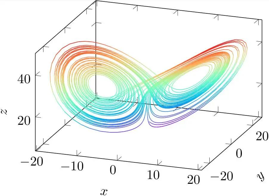
This algorithm can not only effectively avoid falling into local optimality, but also search efficiently on a global scale, showing strong adaptability and flexibility.
Today, we are going to unveil this mysterious and powerful intelligent optimization algorithm-chaos optimization algorithm.
1. The charm of chaos theory
When you think of chaos, you may think ofbutterfly effect——A butterfly flapping its wings in Brazil may trigger a tornado in Texas, USA.

This seemingly absurd metaphor is one of the core features of chaos theory:Sensitivity to initial conditions.
Chaotic systems are extremely sensitive to initial conditions, and even small differences will be quickly amplified during the iterative process, eventually leading to completely different results.
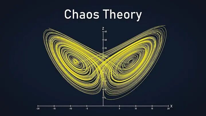
But chaos is not complete disorder. It has a unique "pseudo-randomness" and "ergodicity".
Although a chaotic system seems chaotic, its motion trajectories can be evenly distributed throughout the entire feasible space and will not pass through the same point repeatedly.
This characteristic enables the chaotic system to efficiently explore the entire solution space during the search process and avoid falling into local optima.
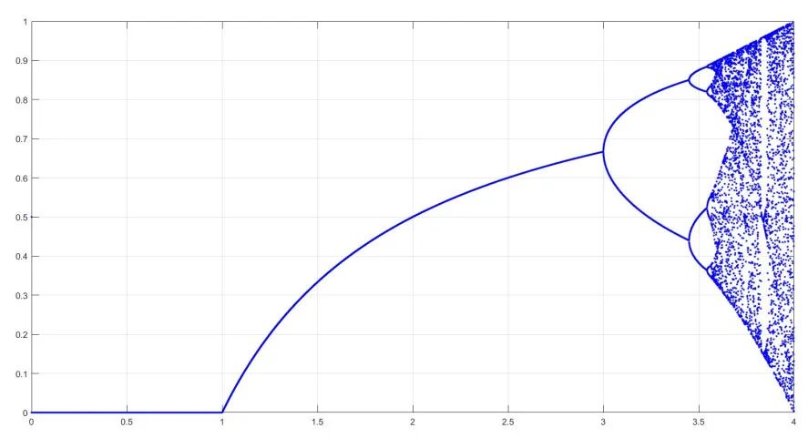
▲ Bifurcation diagram of logistic chaos map
chaos mappingIt is an important application of chaos theory in optimization algorithms. Common chaotic mappings include Logistic mapping and Tent mapping.
-
Logistic mappingIt is a simple nonlinear equation, but its iterative process can produce complex chaotic behavior.
-
Tent mappingWith its linear segmentation characteristics, it shows fast traversal and good randomness.
These chaotic maps provide a powerful source of power for chaotic optimization algorithms.
2. Principle and process of chaos optimization algorithm
The core idea of the chaos optimization algorithm isIntroducing chaotic variables into the variable space of optimization problems, using the ergodicity of chaotic motion to search for the global optimal solution.

It generates chaotic variables through chaotic mapping, and these variables continuously change during the iterative process, thereby driving the efficient search of optimization variables in the solution space.
The implementation steps of the chaos optimization algorithm are as follows:
01 · Initialize chaos variables
First, the chaos variables are initialized according to the size and dimension of the optimization problem.
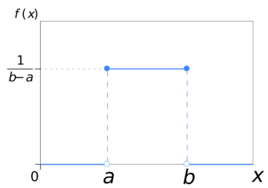
These variables are usually uniformly distributed in the interval [0,1] and are updated iteratively through chaotic mapping.
02 · Chaos variable iteration
Secondly, the chaotic variables are updated using the iterative formula of chaos mapping. For example, the iteration formula of logistic mapping is:
Among them, is the control parameter. When , the system shows chaotic behavior.
Each iteration will generate new chaotic variables, which are converted into optimization variables through a certain mapping relationship.
03 · Optimize search
Then, convert the chaos variables into optimized variables:
Among them, and are the lower and upper bounds of the optimization variables respectively.
Substitute the converted optimization variables into the objective function and calculate its fitness value.
According to the size of the fitness value, the optimal solution is selected as the candidate solution for the current iteration.
04 · Termination condition judgment
Finally, when the preset number of iterations is reached or the fitness value converges, the algorithm terminates and the global optimal solution is output.
3. Case demonstration of chaos optimization algorithm
In order to better understand the working principle of the chaos optimization algorithm, we take the Ackley function as an example for optimization.
01 · Problem Definition
The Ackley function is a classic multimodal function with complex terrain and multiple local minima, and is often used to test the performance of optimization algorithms.
import numpy as npimport matplotlib.pyplot as pltfrom mpl_toolkits.mplot3d import Axes3Dfrom matplotlib.animation import FuncAnimationfrom IPython.display import HTMLimport timeimport math# Set Chinese displayplt.rcParams['font.sans-serif'] = ['SimHei']plt.rcParams['axes.unicode_minus'] = False# Ackley functiondefackley(x): a = 20 b = 0.2 c = 2 * np.pi d = len(x) sum_sq = sum([xi**2for xi in x]) sum_cos = sum([np.cos(c * xi) for xi in x]) term1 = -a * np.exp(-b * np.sqrt(sum_sq / d)) term2 = -np.exp(sum_cos / d) return term1 + term2 + a + np.exp(1)
02 · Algorithmic Modeling
When implementing the chaos optimization algorithm, we chose Logistic chaos mapping as the generation method of chaotic sequences.
# Logistic Chaos Mappingdeflogistic_map(x, mu=4.0): return mu * x * (1 - x)#Chaos optimization algorithmdefchaos_optimization(obj_func, dim, lb, ub, max_iter, chaos_iter=1000): """Parameters:- obj_func: objective function- dim: problem dimension- lb: lower bound- ub: upper bound- max_iter: maximum number of iterations- chaos_iter: number of chaos iterations """#Initialize chaos variables chaos_vars = np.random.rand(dim) # Generate chaotic sequence chaos_sequence = [] for _ inrange(chaos_iter): chaos_vars = logistic_map(chaos_vars) chaos_sequence.append(chaos_vars.copy()) chaos_sequence = np.array(chaos_sequence) # Map the chaotic sequence to the search space search_points = lb + (ub - lb) * chaos_sequence # Evaluate initial solution fitness = np.array([obj_func(p) for p in search_points]) best_idx = np.argmin(fitness) best_position = search_points[best_idx].copy() best_fitness = fitness[best_idx] # Record history history = { 'positions': [search_points.copy()], 'best_position': [best_position.copy()], 'best_fitness': [best_fitness], 'current_iter': [0] } # Algorithm starts print("="*50)print("Chaos Optimization Algorithm (COA) starts running")print(f"Search space dimension: {dim}")print(f"Search range: [{lb}, {ub}]")print(f"Maximum number of iterations: {max_iter}")print(f"Number of chaos iterations: {chaos_iter}")print(f"Initial best fitness: {best_fitness:.6f}") print("="*50) time.sleep(1) # Secondary carrier search foriterinrange(max_iter):# Narrow the search scope current_lb = np.maximum(lb, best_position - (ub - lb) * 0.9**(iter+1)) current_ub = np.minimum(ub, best_position + (ub - lb) * 0.9**(iter+1)) # Generate a new chaotic sequence new_chaos_vars = np.random.rand(dim) new_search_points = [] for _ inrange(chaos_iter): new_chaos_vars = logistic_map(new_chaos_vars) new_point = current_lb + (current_ub - current_lb) * new_chaos_vars new_search_points.append(new_point) new_search_points = np.array(new_search_points) # Evaluate new solution new_fitness = np.array([obj_func(p) for p in new_search_points]) current_best_idx = np.argmin(new_fitness) current_best_position = new_search_points[current_best_idx].copy() current_best_fitness = new_fitness[current_best_idx] # Update optimal solution if current_best_fitness < best_fitness: best_position = current_best_position.copy() best_fitness = current_best_fitness # Record history history['positions'].append(new_search_points.copy()) history['best_position'].append(best_position.copy()) history['best_fitness'].append(best_fitness) history['current_iter'].append(iter+1) # Print progress ifiter % 10 == 0oriter == max_iter-1:print(f"Iteration {iter+1:3d}/{max_iter} | Current best fitness: {best_fitness:.6f}") print("="*50)print("Optimization completed!")print(f"The best solution found: {best_position}")print(f"Best fitness value: {best_fitness:.6f}") print("="*50) time.sleep(1)print("Generate visual results...") time.sleep(1) return history
02·Result visualization
In order to display the optimization process of the chaos optimization algorithm more intuitively, we drew 3D surface plots, 2D contour plots and convergence curves through Matplotlib.
# Parameter settingsdim = 2lb = -5ub = 5max_iter = 50chaos_iter = 500# Run the algorithmhistory = chaos_optimization(ackley, dim, lb, ub, max_iter, chaos_iter)# Prepare data for visualizationx = np.linspace(lb, ub, 100)y = np.linspace(lb, ub, 100)X, Y = np.meshgrid(x, y)Z = np.zeros_like(X)for i inrange(X.shape[0]): for j inrange(X.shape[1]): Z[i,j] = ackley([X[i,j], Y[i,j]])#Create visualization graphicsfig = plt.figure(figsize=(18, 6), dpi=100)fig.suptitle('Chaos optimization algorithm optimization process', fontsize=16)# Unify sub-picture sizegs = fig.add_gridspec(2, 3, width_ratios=[1, 1, 1], height_ratios=[1, 1])# 3D surface plotax1 = fig.add_subplot(gs[:, 0], projection='3d')surf = ax1.plot_surface(X, Y, Z, cmap='viridis', alpha=0.6)fig.colorbar(surf, ax=ax1, shrink=0.6, aspect=10, label='function value')scatter = ax1.scatter([], [], [], c='red', s=10, alpha=0.5, label='Chaos search point')best_scatter = ax1.scatter([], [], [], c='blue', marker='*', s=200, label='best solution')ax1.set_title('3D function surface and chaos search', fontsize=12)ax1.set_xlabel('x1', fontsize=10)ax1.set_ylabel('x2', fontsize=10)ax1.set_zlabel('f(x)', fontsize=10)ax1.legend(loc='upper right', fontsize=8)# 2D contour plotax2 = fig.add_subplot(gs[:, 1])contour = ax2.contourf(X, Y, Z, levels=50, cmap='viridis')fig.colorbar(contour, ax=ax2, shrink=0.6, aspect=10, label='function value')scatter2d = ax2.scatter([], [], c='red', s=10, alpha=0.5, label='Chaos search point')best_scatter2d = ax2.scatter([], [], c='blue', marker='*', s=100, label='best solution')search_area = plt.Rectangle((0,0), 0, 0, color='yellow', alpha=0.3, label='current search area')ax2.add_patch(search_area)ax2.set_title('2D contours and chaos search', fontsize=12)ax2.set_xlabel('x1', fontsize=10)ax2.set_ylabel('x2', fontsize=10)ax2.legend(loc='upper right', fontsize=8)# Convergence curveax3 = fig.add_subplot(gs[0, 2])convergence_line, = ax3.plot([], [], 'b-', linewidth=2, label='best fitness')current_point = ax3.scatter([], [], c='red', s=50, label='current value')ax3.set_title('Fitness convergence curve', fontsize=12)ax3.set_xlabel('number of iterations', fontsize=10)ax3.set_ylabel('Fitness value', fontsize=10)ax3.grid(True, linestyle='--', alpha=0.6)ax3.set_xlim(0, max_iter)ax3.set_ylim(0, max(history['best_fitness']))ax3.legend(loc='upper right', fontsize=8)# Parameter displayax4 = fig.add_subplot(gs[1, 2])ax4.axis('off')info_text = ax4.text(0.1, 0.5, '', fontsize=10, bbox=dict(facecolor='white', alpha=0.8))plt.tight_layout()#Modify update functiondefupdate(frame):# Only display some points to avoid being too dense display_points = history['positions'][frame][::10] # Update 3D image current_z = np.array([ackley(p) for p in display_points]) scatter._offsets3d = (display_points[:,0], display_points[:,1], current_z) best_pos = history['best_position'][frame] best_z = ackley(best_pos) best_scatter._offsets3d = ([best_pos[0]], [best_pos[1]], [best_z]) # Update 2D graph scatter2d.set_offsets(display_points) best_scatter2d.set_offsets([best_pos]) #Initialize search area current_iter = history['current_iter'][frame] if current_iter == 0:# Use the global search scope for the first frame current_lb = np.array([lb, lb]) current_ub = np.array([ub, ub]) else:#Narrow the search range in subsequent frames current_lb = np.maximum(lb, best_pos - (ub - lb) * 0.9**current_iter) current_ub = np.minimum(ub, best_pos + (ub - lb) * 0.9**current_iter) # Update the search area display search_area.set_xy((current_lb[0], current_lb[1])) search_area.set_width(current_ub[0] - current_lb[0]) search_area.set_height(current_ub[1] - current_lb[1]) # Update convergence curve x_data = range(current_iter+1) y_data = history['best_fitness'][:current_iter+1] convergence_line.set_data(x_data, y_data) current_point.set_offsets([[current_iter, history['best_fitness'][current_iter]]]) # Update text informationinfo = f"Number of iterations: {current_iter}\n"info += f"Best fitness: {history['best_fitness'][current_iter]:.6f}\n"info += f"Best position: [{best_pos[0]:.4f}, {best_pos[1]:.4f}]\n"info += f"Search area: [{current_lb[0]:.2f}, {current_ub[0]:.2f}] x [{current_lb[1]:.2f}, {current_ub[1]:.2f}]\n"info += f"Number of chaos iterations: {chaos_iter}\n"info += f"Current search points: {len(history['positions'][frame])}" info_text.set_text(info) return scatter, best_scatter, scatter2d, best_scatter2d, search_area, convergence_line, current_point, info_text# Create animationani = FuncAnimation(fig, update, frames=len(history['positions']), interval=500, blit=True)# Show animationplt.close()HTML(ani.to_jshtml())
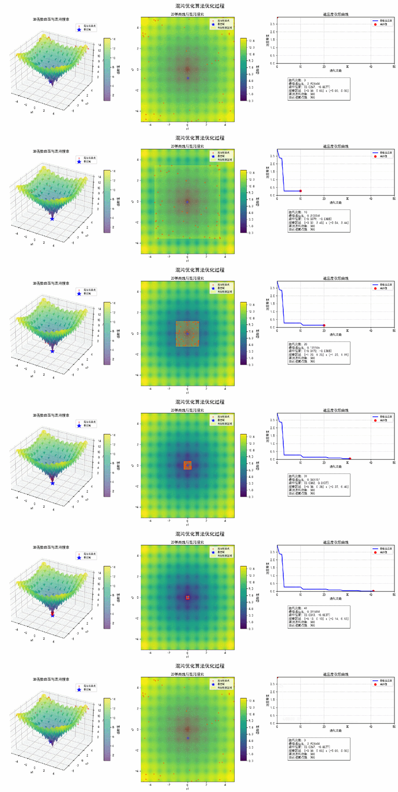
Result display|Result output
After 50 iterations, the chaos optimization algorithm successfully found the global optimal solution of the Ackley function.
Conclusion
Chaos optimization algorithm has shown great potential in the field of intelligent optimization with its unique chaos theory foundation, powerful global search capability and wide range of application fields.
It can not only solve complex optimization problems, but can also be combined with other optimization algorithms to achieve more efficient optimization searches.
Note: It is not stated in the article that the pictures are all from the Internet
Machine-translated from the Chinese original 混沌优化算法(COA):从理论到实践的探索之旅 (published 2025-06-26). WeChat original ↗