【Abstract】Solving the vehicle routing problem (VRP) is an important task for many industrial applications. Although VRPs have traditionally been studied in the field of operations research (OR), recently they have become the subject of extensive work in the machine learning (ML) community. Both the OR and ML communities are starting to integrate ML into their approach, but in very different ways. While the OR community mainly relies on simple ML methods, the ML community often uses deep learning but cannot surpass the OR baseline. To address this gap, the EURO Meets NeurIPS 2022 Vehicle Routing Competition brings together the OR and ML communities as a joint effort from several previous competitions to tackle challenging VRP variants on real-world data provided by ORTEC, a leading provider of vehicle routing software. The challenge focuses on "classic" deterministic VRP with time windows (VRPTW) and a dynamic version where new orders arrive within a day. More than 50 teams submitted solutions during the 13-week submission period, competing not only for the best performance on the competition problem, but also for longest dominance on the leaderboard. The competition's goals were achieved, with operations research and state-of-the-art technology playing an important role in several winning entries.
【Key words】Machine learning, combinatorial optimization, stochastic optimization, vehicle routing problem with time window, dynamic scheduling problem
*For details, please click "Read the original text" in the lower left corner of the article.
Total text: 8588 words
Estimated reading time: 14-22 minutes

01 · Introduction
Every day, millions of trucks and other vehicles perform deliveries or services around the world. Finding the best routes for these vehicles is critical for companies to reduce costs and environmental impact. The vehicle routing problem (VRP) is a generalization of the well-known traveling salesman problem (TSP) and has therefore been the focus of significant research activity. In VRP, the goal is to find a route for a set of vehicles and a set of customers such that each customer is visited once by one of the vehicles and the total distance traveled (or travel cost incurred) is minimized. Many extensions of VRP have been studied in the literature (Vidal et al., 2020), including, for example, time windows (called VRPTW), which require delivery to customers within a specific time period, as well as random variables (e.g., uncertain duration of travel between customers) or dynamic variables that change over time (Pillac et al., 2013).
VRP has traditionally been studied in the field of operations research (OR), where solution methods mainly rely on searching the space of feasible solutions using exact methods or heuristic methods (Laporte et al., 2014; Poggi and Uchoa, 2014; Costa et al., 2019). In recent years, this problem has also attracted the attention of machine learning (ML) researchers (Nazari et al., 2018; Kool et al., 2018, Kwon et al., 2020; Hottung et al., 2020, Xin et al., 2021b; d O Costa et al., 2020), da Costa et al., 2021, Xin et al., 2021a; Kool et al., 2022b; Bai et al., 2021; Choo et al., 2022), who developed various methods using deep neural networks (DNN), through optimal solutions or using reinforcement learning. While these techniques differ in terms of problem-specific components and general search schemes, most of them currently do not surpass state-of-the-art OR solution strategies, which are often based on fast local search and employ additional meta-heuristic strategies to guide the exploration of the solution space.
Work on the vehicle routing problem proceeds very differently between the ML and OR communities, sometimes using different solution evaluation practices, hardware, and benchmarks, with different emphasis on speed and solution quality, and with different perspectives on application-oriented versus method-oriented work. With this in mind, the EURO Meets NeurIPS 2022 vehicle routing competition aims to bring the two communities together to solve the same routing problems and benchmarks, thus promoting cross-pollination between regions. The competition is a joint effort of the VeRoLog competition (Gromicho et al., 2019), the European Vehicle Routing and Logistics Optimization Working Group (VeRoLog), the EURO Data Science Working Group Satisfaction Optimization (DSO) of the IJCAI AI 4TSP competition (Zhang et al., 2023), and the DIMACS Implementation Challenge (Archetti et al., 2021) organized by the Center for Discrete Mathematics and Theoretical Computer Science (DIMACS). The competition involves solving static and dynamic versions of VRPTW, with the goal of providing the OR and ML community with the opportunity to leverage learning algorithms and advanced methods. In addition to the first three competitions, other recent examples of relevant competitions are the Amazon Last Mile Routing Challenge (Merch´an et al., 2022) and the CEC-12 Electric Vehicle Routing Problem Competition (Mavrouniotis et al., 2020).
This article provides an overview of the competition and lessons learned. We define the competition problem in Section 2, describe the schedule setting in Section 3, summarize the final team's methods in Section 4, discuss the final results in Section 5, and review in Section 6.
02 · Problem Statement
VRPTW has long been the focus of operations research researchers (Kallehauge et al., 2005) as it appears in multiple application contexts and problem variants, such as home medical routing (Fikar and Hirsch, 2017), technician routing (Paraskevopoulos et al., 2017), and integrated truck-drone delivery (Chung et al., 2020). We chose VRPTW and its dynamic variants for competition because the problems are canonical and easy to model, but finding low-cost solutions is challenging due to time window limitations of customer visits and capacity constraints of vehicles. Apart from this, the static and dynamic versions of VRPTW have not received a lot of work from the machine learning community, which makes them a prime target to bring the machine learning community closer to real-world applications and encourage the OR community to use more advanced machine learning methods. In the following, we formalize VRPTW, starting with the standard (static) version and then its dynamic variants.
Static question setup:VRPTW is a constrained variant of Capacity Constrained VRP (CVRP), where each customer is required to deliver within a specified interval, called a time window. The static problem is defined as follows. The VRPTW problem instances considered in this competition consist of n locations(a warehouse and a set of n-1 customers), an n×n matrix D that specifies the travel time between each pair of locations(in seconds) (it represents the actual road travel time in seconds and is neither Euclidean nor symmetric), the product demand of each customer iqiand the maximum quantity Q that the vehicle can carry, also known as the vehicle's capacity.
Each customer represented by node i also has a service duration si and a time window [ei,li], where ei<li, service/delivery must start within this time window, siRepresents the time required to provide service to customer i. The vehicle is allowed to arrive at the customer's location before the time window begins, but must wait until the delivery window begins before delivery can begin. Deliveries cannot start after the time window has closed. In this way, competitors treat the time window constraints as hard constraints. There is no limit to the number of vehicles available.
A feasible solution for VRPTW consists of a set of routes starting and ending at a parking lot, such that each customer is accessible on a route within a specified time window and the total demand assigned to a route does not exceed the vehicle capacity Q. The goal is to find a feasible solution that minimizes the total driving time for all routes. Please note that vehicle numbers, service times and wait times are not the goals of this competition. The problem definition follows the convention used in the recent DIMACS VRPTW challenge, except that the matrix D is not Euclidean and the number of vehicles is infinite. Through these conventions, the feasibility of the problem is guaranteed even in dynamic environments (see next section).
Dynamic question settings:For the dynamic variant of the problem, requests arrive at different one-hour slots throughout the day. The solver can choose which requests to dispatch in the current time period, which requests must create feasible routes, and which requests to defer to be merged with new requests that may arrive later. Some requests are "must do" requests and must be sent within the current time period because delaying them to the next time period would make their time window unfeasible. During the last period, all requests must be executed. From the data of the static VRPTW instance, the location, demand, service time and time window of the requests in each time period are uniformly sampled, and then the requests with infeasible time windows are filtered.
03·Contest details
The competition is divided into a qualifying stage and a final stage. The top 10 entries in the qualifying stage will be tested on 100 hidden test instances. During the qualifying phase, results will be displayed on the public leaderboard. During the qualification phase, submissions for static questions are limited to 3 to 8 minutes, depending on the size of the instance, and dynamic questions are limited to 1 minute each. In the final phase, this time limit increases to 5 to 15 minutes and 2 minutes per time period respectively.
In the quickstart repository, a public dataset of 250 static VRPTW instances is provided. These are real examples provided by ORTEC, using anonymized data from a food delivery service in the United States. These instances contain between 200 and 900 customers. From these static instances, the environment creates dynamic instances by sampling 100 requests from the static client set over 5 to 9 time periods (afterwards filtering requests with infeasible time windows), depending on the instance. Public instances and provided environments can be used to develop solvers or train machine learning models.
All examples are provided in VRPLib format following the convention used by LKH3. Since static problems are a special case of dynamic problems, solvers are evaluated for both static and dynamic problem variants using the same protocol. For this protocol, we used an environment implemented in Python that follows the OpenAI gym interface (Brockman et al., 2016). Here, the environment accepts an action and returns an observation, a reward, a flag indicating whether the environment is complete, and additional information. The term comes from reinforcement learning, where the solver can be thought of as an agent interacting with the environment. In this terminology, observations define the VRPTW/request selection problem for each epoch, actions are solutions that define a set of scheduled routes, and rewards are the negative value of the cost (driving duration) of the solution (set of scheduled routes) for that epoch. Solving a problem until completion (with multiple periods) can be called an episode of the environment.
3.1 Baseline
We provide participants with some baselines when developing solvers.
Static baseline:As a baseline for static variants, we provide an implementation of the Hybrid Genetic Search (HGS) algorithm (Vidal et al., 2012; Vidal, 2022), which combines a genetic algorithm with local search. HGS and its extensions have been used to produce state-of-the-art results for many variants of the vehicle routing problem (Vidal et al., 2013, 2014; Vidal, 2022). Specifically, the baseline we provide is an extension of HGS-CVRP (Vidal, 2022) used by Kool et al. (2022a) to win the VRPTW track of the DIMACS Implementation Challenge and can therefore be considered state-of-the-art. This implementation uses the strategy of Vidal et al. (2013). Efficiently evaluate time window constraints via search. Furthermore, compared to HGS-CVRP, it includes additional crossovers from Nagata et al. (2010). Dynamic parameters for population and community size management, as well as some code optimizations.
Dynamic strategy:So far, all vehicle routing variants solved using HGS have been static. In our case, a static solver is extended to handle the required dynamic requests, choosing which requests should be served at any given time period. Such expansion is not easy and requires additional customer selection strategies.
To select which requests to dispatch in each time period, we provide three initial simple strategies in the quickstart repository:(1) Greed:Every available request will be dispatched within the current time period. This means that all requests are included in HGS route optimization;(2) Laziness:Only requests that must be sent will be sent. A must-go request is one that cannot be deferred to the next time period due to a time window violation (as indicated by the environment); and(3) Randomly:Randomly select requests to schedule during the current time period: each request is scheduled independently with a 50% probability. Please note that requests that must be submitted in order to obtain a workable solution will always be included.
Additionally, during the competition we added two additional baselines using machine learning:(1) Supervision:Create an example using Oracle Solver (using future information) to train a neural network to predict requests sent by Oracle, and(2)DQN:Deep Q-Network (DQN) (Mnih et al., 2013) agents are trained using reinforcement learning to select requests by repeatedly interacting with the environment. The machine learning baseline is for illustrative purposes only and does not extend beyond the greedy baseline. Together, these baselines provide preliminary comparison results and are included in public rankings, but not as official participants.
3.2 Rating and Submission System
Teams are asked to submit code that can generate a solution given an instance: for example, a hand-designed heuristic, or a policy trained with reinforcement learning. This allows us to test submitted code on hidden test instances, which we use to determine the final winner based on the quality of the solution on those instances. As stated in the problem statement, the score for each instance is calculated as the total time traveled by all vehicles (i.e. not including service or waiting time). For this reason, smaller fractions are preferable.
The scores for each instance of the hidden instances of the static problem across all teams and the hidden instances of the dynamic problem across all teams were averaged, resulting in separate rankings of teams for the two problem variants. Each team's two rankings are then averaged to arrive at each team's final ranking for the entire competition. This ensures that both questions are weighted equally regardless of the actual score. In the event of a tie, the scores themselves are averaged, not the rankings.
To enable code submissions, we use the Codalab Competition platform and provide instructions for participants in the quickstart repository. The code is executed within an Apptainer/Singulity container based on a Dockerfile to ensure the same environment is provided to all participants so that they can reproduce it for testing. The environment has one CPU core (Intel(R) Xeon(R) Gold 5118 [email protected]), one GPU (Nvidia TitanRTX 24GB) and 32GB RAM.
3.3 Prizes
We offer the following prizes to the winners, totaling more than 5000 €.
1. Best performance: 2022/750/500 € Rank 1st/2nd/3rd
2. Jury Prize: 250 €
3. Young Talent Award: 250 €
4. Leaderboard prizes: total €1300
The top three awards will be scored according to the final hidden dataset ranking criteria described in Section 3.2. To further encourage innovative ideas, even if they do not lead to optimal performance, the organizers will, at their discretion, award a "Jury Prize" to an approach that provides a novel methodological idea. For this award, we look for an approach that: (1) provides a novel solution; (2) uses machine learning; (3) achieves good performance within the allotted time; and (4) does not win first place.
The Young Talent Award is awarded to the best performing team consisting exclusively of students and/or PhD students. Finally, the leaderboard bonus is 50/30/20 €, awarded weekly to 1/2/3 numbers on the leaderboard to encourage early competition.
04 · Summary of team contributions
Each finalist team described their approach in a short paper, which was presented at the final workshop (see Section 6). Papers and presentation slides have been posted on the competition website5. We outline the finalists' contributions here.
Kleopatra Jungel et al. (2022): Improved HGS for static variants by reducing some randomization steps and implementing a caching mechanism for immutable routes in local search iterations. For dynamic problems, they implemented a parameterizable HGS (PC-HGS) prize collection variant that jointly optimizes the selection of scheduling requests and routes based on a set of prizes that represent preferences for scheduling requests in the current epoch. The optimal reward is unknown a priori, but a machine learning model is trained to predict the reward, using a loss function to encourage PC-HGS results to approach the expected oracle solution (see baseline).
OptiML van Doornetal. (2022): Simplified implementation of the baseline human genome system by removing the ordered crossover, initial structure, and growing community/population components introduced by Kool et al. (2022a). shown in . They added diversity criteria to the parent selection step, made code optimizations for local searches, and made extensive adjustments to parameters. For dynamic problems, their approach simulates multiple scenarios of future requests, for which they optimize routing using a solver as an oracle (see baseline). May-go requests that are frequently combined with must-go requests in simulations are also marked as must-go, and this process is repeated several times to define the final set of requests to be dispatched. This set is then optimized using a static solver and all routes with at least one (original) must-execute request are dispatched.
Team SB Kwon et al. (2022): Adjusted HGS parameters and generalized binary tournaments to k-way tournaments, where k is automatically adjusted so that higher fitness individuals are selected more frequently if a new optimal solution has been found recently. Additionally, to encourage diversity, individuals are removed from the population after a certain number of offspring and a warm restart mechanism. The dynamic variant uses two neural networks: one to predict the priority of requests and another to select which requests must be dispatched. These are used in the HGS algorithm, with modified targets, to select requests, weighing priorities against extra distance. Both networks are trained using reinforcement learning.
HustSmart Li et al. (2022): Added EAX crossover to HGS and added a SISR algorithm to optimize the solution each time a new optimal solution is found. For dynamic problems, they compute a heuristically defined penalty score for each request and use an OR tool to solve VRPTW while allowing access to be dropped at the cost of penalty. This results in a set of requests, the routing of which is then further optimized using the HGS algorithm.
Miles To Go Before We Sleep Reese et al. (2022): Made multiple performance improvements to the HGS code for static problems and tuned parameters on different subsets of training instances. For a dynamic variant of the problem, they implemented two heuristics for selecting requests to send for possible execution of orders based on their (basic) closeness to the order that must be executed. Use HGS to optimize a given selected route.
ORBerto Hood Hildebrandt et al. (2022): HGS parameters are tuned for the static variant of the problem and the set of scheduling requests for the dynamic variant is optimized across a sampled set of future scenarios. To do so, they defined a single integration problem considering all scenarios and solved it using a column generation process. Optimized routing of result request sets using HGS.
HowToRoute Mesa et al. (2022): Reduces the frequency of the reinforcement process and implements adjusted crossovers in the HGS algorithm. For the dynamic variant, they sent possible go requests that were close to the must-go requests and found a solution using HGS. They then applied a method to remove possible requests from the route (that would be deferred) if this lowered the average cost of requests in the route. The final selection was further refined using HGS.
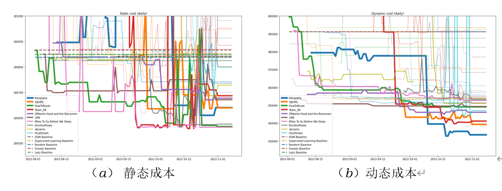
Figure 1: Static and dynamic results of the qualifying phase of the competition
Kirchhoffslaw Ao and Zong (2022): HGS parameters were tuned for the static variant of the problem and a neural network was trained using reinforcement learning to select scheduling requests for the dynamic variant. The operations correspond to whether an order should be selected, and the final reward is calculated by comparing the final cost after running HGS on the selected request each epoch with the final cost of the greedy baseline method.
UPB Dieter (2022): Focuses on the dynamic variables of the problem and implements a regret strategy that uses available information about the request distribution to analytically calculate the regret value for each walkable request: improvements that might be missed when the request would be scheduled immediately. Requests with regret values below the threshold are sent immediately and optimized using HGS.
dynamo GhannamandGleixner (2022): Added an additional HGreX crossover to HGS to resolve static issues. For the dynamic variant, they adapted HGS to allow a subset of requests to be included in the optimization, where the average cost of the order (total driving time divided by the number of requests) was targeted. Penalties ensure that orders must be placed immediately and support additional delay terms, including requests for early end of the time window.
05 · Results
Figure 1 shows the results on the public leaderboard for static and dynamic problem variants for different teams during the qualifying phase. The graphs are not strictly reduced as the results from different evaluations may differ slightly, but for both problem variants we see a clear trend towards improving results as the competition progresses. The team's average ranking on the static and dynamic questions determines the overall ranking on the leaderboard, as shown in Figure 2. The number of participants on the leaderboard steadily increased during the competition, with some finalists only reaching the top 10 of the public leaderboard at the end of the qualifying phase.
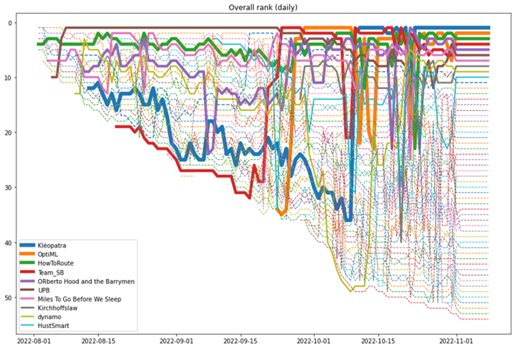
Figure 2: Leaderboard rankings in the qualifying stage of the competition
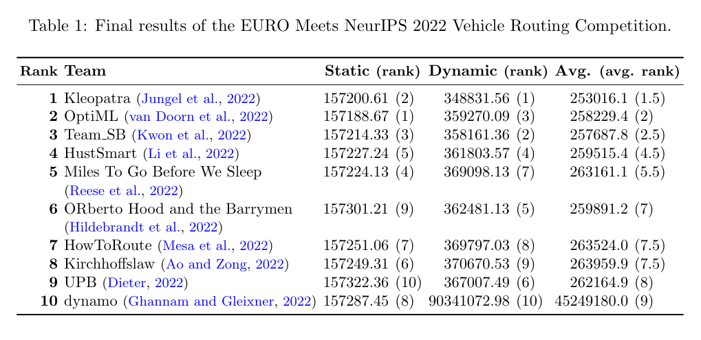
The top 10 on the public leaderboard determines the finalists, who are comprehensively evaluated in the final stages of the competition. This is done using a hidden test set, which consists of 100 instances that are solved in both static and dynamic variants with longer running times (see Section 3). Table 1 shows the results for the finalists, where teams are ranked based on their average ranking on the static and dynamic variants of the problem. Team Kleopatra (Jungel et al., 2022) took first place, placing first on the dynamic problem and second on the static problem, winning €2022. The OptiML team (van Doorn et al., 2022) placed first on the static problem, third on the dynamic problem, and second overall, winning €750. Team SB (Kwon et al., 2022) received third place and €500 for placing third on the static problem and second on the dynamic problem. Overall, we observed a strong correlation between each team's performance on the static and dynamic variants of the problem, suggesting that the teams were able to allocate their efforts well between the two problems.
The Jury Prize was awarded to the SB team for their outstanding results using an innovative approach based on machine learning. The Young Talent Award was awarded to the Kleopatra team. Finally, leaderboard awards for entering the top three public leaderboards during the qualification phase were awarded to the UPB, Kleopatra, SB, 4pd vrp and OptiML teams.
All real data used during the competition, including the hidden dataset used for the final evaluation, has been made available under a CC BY-NC 4.0 license in the competition GitHub repository. We hope that this dataset will continue to be used as a real-world benchmark. For the purpose of verifiability and reproducibility, all settings used for the final evaluation and the single solution found by the finalists. In addition, the solver is released, along with a notebook that reproduces the final results table. Most finalist teams have published their codes, which are linked on the competition website.
06 · Review
In the end, nearly 150 teams registered through the website, and 50 of them submitted final entries. During the qualification review phase, more than 800 submissions were submitted. 180 people joined the Slack workspace and around 4500 messages were exchanged there, so this is actively used to communicate with participants. Participants include researchers from the operations research and machine learning communities, as well as many teams from academia and some industry players. Attendees come from all over the world.
The NeurIPS wrap-up workshop was held as a virtual conference on December 7, 2022. About 30 people took part in the competition, including competition organizers and members of the 10 final teams. The recording can be found on the competition website.
In hindsight, (real world) datasets for static problems contain many instances that are too small to improve upon the HGS baseline, since optimal or near-optimal solutions are always found in short CPU time. Nonetheless, this part of the challenge still leads to useful methodological and practical developments. In particular, the software developed by OptiML, the team ranked first in static variants, has been released as PyVRP, a state-of-the-art open source VRPTW solver that can be easily used from Python. This will help machine learning researchers build and contribute state-of-the-art OR solvers on future vehicle routing problems.
The dynamic variant of the problem achieves very significant progress beyond the baseline strategy compared to the static variant. All the best methods use machine learning as a key component of their winning strategies. This shows that machine learning is not only promising in the future, but can already compete with other methods on dynamic optimization problems.
The motivation for having two problem variables, but scoring participants on their combined performance, is to reward versatile approaches that work on both variables and to ensure that efforts are directed both at improving static performance and at dealing with the dynamic aspects of the problem. In practice, most teams implemented specific solution strategies for both variants, and in a few cases only adjusted the baseline algorithm parameters for the static variant.
From a technical perspective, the Codalab platform enables us to evaluate code submissions, but we needed to make many adjustments to make it work for our use case. Since our evaluation requires a GPU, we had to hook up our own compute workers, and while Codalab provides a Docker image to support this use case, it assumes running a dedicated worker 24/7, which wastes (GPU) compute resources because the submission queue will be empty most of the time. In order to evaluate submissions as jobs on a shared machine cluster, we had to 1) switch to Apptainer/Singulity (because Docker requires unavailable root permissions), 2) adjust the Worker script to terminate when the queue is empty, and 3) set up a separate external monitoring script to start jobs when there are new submissions in the queue.
In addition to the evaluation, there are some additional challenges: the Codalab leaderboard does not calculate the ranking correctly, so we publish a correct leaderboard, which will be automatically updated on our own competition website. In the future, given the combination of challenges, we will look into other platforms such as Kaggle or AICrowd. Nonetheless, the submission platform with live leaderboards played a vital role in the competition, with participating teams telling us they refreshed the page multiple times a day. Public results encourage teams to perform better and participate actively early in the competition, and leaderboard prizes are an added incentive.
07 · Conclusion
As organizers of the competition, we are pleased to see that this competition has successfully brought together AI and OR researchers to generate new approaches that advance state-of-the-art ML and OR technologies to solve both static and dynamic versions of VRPTW. Additionally, we provide examples from the competition as real-world benchmarks that researchers can use to test new methods. All developed baseline methods and implementations by many participants are also publicly available. In the future, the organizing team will continue to work hard to bring the OR and AI communities together to solve relevant real-world optimization problems.
Acknowledgments
We would like to thank ORTEC for sponsoring the majority of the prize pool, as well as EURO VeRoLog and the DSO working group who provided additional support for the jury and the Young Talent Awards. The computing infrastructure used in the competition is generously sponsored by the HPC Laboratory of Eindhoven University of Technology. Finally, we would like to thank EURO and the NeurIPS conference for their support in organizing this competition.
*References are omitted. For details, please click "Read the original text" in the lower left corner of the article.

Translation | Yizhe Technology
Machine-translated from the Chinese original The EURO Meets NeurIPS 2022 Vehicle Routing Competition (published 2025-02-25). WeChat original ↗