Intelligent path planning system solution based on OR-Tools

This is a multi-factory logistics distribution path planning system solution based on Google OR-Tools.

The system uses the CVRPTW algorithm to solve the vehicle routing problem with capacity and time windows. It controls the solution within 20 minutes through partition clustering, solution time box and historical solution warm start, and uses Kubernetes to implement parallel computing in 20 factory areas. At the constraint level, a pluggable DSL engine is designed to support configuration management of constraints such as capacity, time window, and vehicle model restrictions.

A highlight of the solution is the optimization closed loop driven by historical data: learning driver experience paths through GPS trajectories, counterfactual deduction to quantify the benefits of constraint relaxation, and incorporating potential customers into simulation planning to assist in sales expansion.

1. Overall architecture design

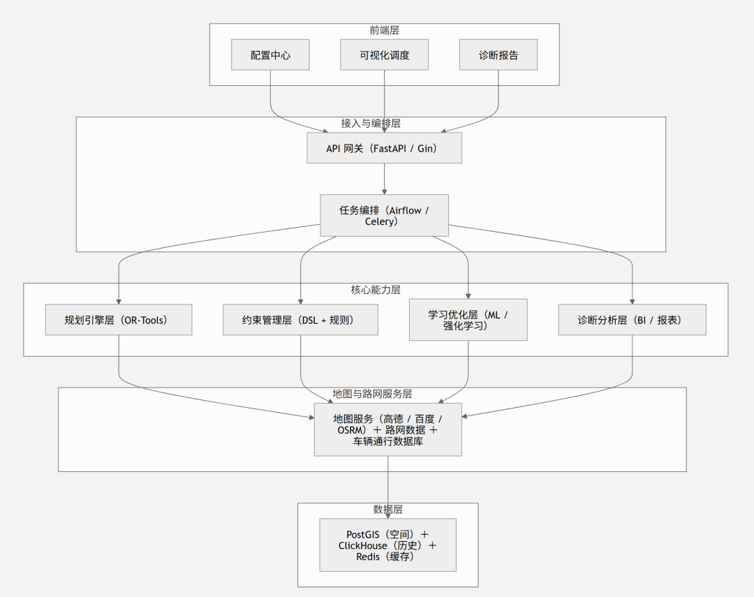
2. Detailed explanation of sub-module scheme

1·Planning operation efficiency (one-click generation & parallel) algorithm body

OR-Tools RoutingModel + CVRPTW (vehicle routing problem with capacity and time window), using PATH_CHEAPEST_ARC first solution + GUIDED_LOCAL_SEARCH meta-heuristic.

20 minutes constraint reached

The POC stage can basically achieve solution within 20 minutes. If there is a situation where some orders are too large, consider the following ways to split and simplify:

• Hierarchical solution:First cluster the partitions (K-Means/DBSCAN by geography + time window), and then solve each sub-region independently → the complexity is reduced from O(n²) to O((n/k)²·k).

• Solving time box:search_parameters.time_limit.seconds = 900 (15min hard constraint) + solution_limit early stop.

• First solution acceleration:Use the historical optimal solution as warm start (ReadAssignmentFromRoutes).

20 factories in parallel

• Kubernetes Job/Celery Worker Pool, independent process isolation per factory (OR-Tools single instance thread safety limited).

• Each Pod reserves 4C8G, with a total of 20 Pods running in parallel; the scheduler distributes tasks uniformly, and MQ recycles the results.

One click trigger

Scheduled tasks (T-1 22:00 the next day) automatically pull orders → verify integrity → schedule and solve → store results → push.

2 · Constraint configuration capabilities and intelligent paths

2.1 Constraint DSL engine

The abstract constraint is a pluggable component (strategy pattern), and the background configuration is:

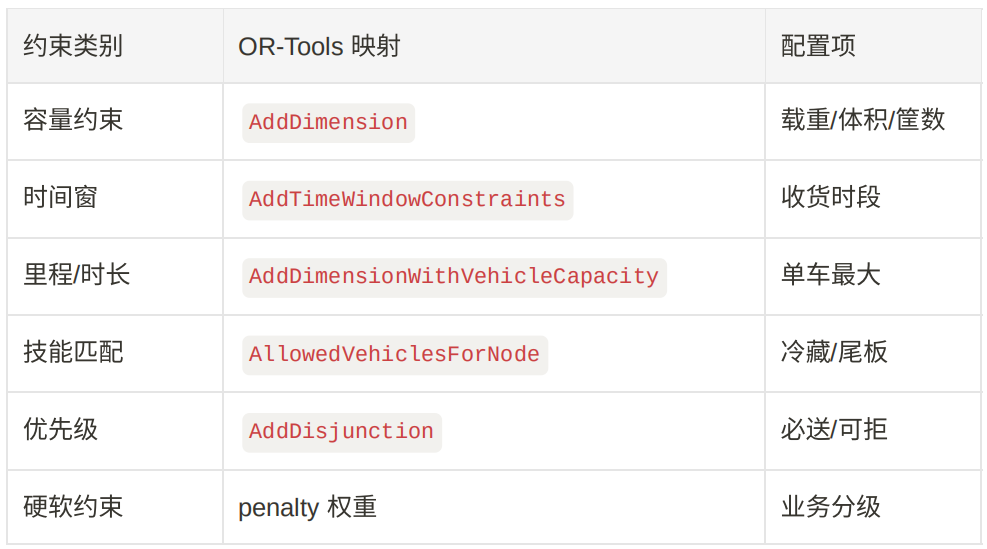
• New constraint process:Create a new business party in the configuration center → system generates JSON Schema → engine dynamic note RoutingModel, no release required.

2.2 Vehicle models avoid impassable roads

• Road network attribute marking:Access the AutoNavi truck route API (requires enterprise-level AutoNavi API), and each edge is marked with max_height/width/weight/tonnage.

• Dynamic cost matrix:Filter the road network according to vehicle types → Use OSRM to generate customized distance_matrix → Feed to OR-Tools.

• CRM linkage:The customer's delivery point label (underground garage/narrow alley/no traffic at night) is used as a node constraint. When planning, choose to match the vehicle model or adjust the time window.

2.3 Historical driver route learning

• Deviation analysis:Compare planned routes vs. GPS trajectories using Fréchet distance to identify "experience shortcuts" that drivers often take.

• Cost correction:Discount the edge cost of the experience path (multiplied by 0.9~0.95), and you will naturally choose it next time.

• Calibration time:Statistics of actual traffic speed according to (road section, time period, vehicle type) dimensions, replacing the default speed table.

  
  

3·Dynamic adjustment of orders

3.1 Multiple scene changes

• Incremental mode (the original line remains unchanged):Treat new/cancelled points as local disturbances, use CloseModelWithParameters of OR-Tools + fix the locked path + only optimize the changed nodes → return in seconds.

• Full weight planning:Go through the entire process.

3.2 Upstream and downstream balance

• Introducing the dimension of factory capacity constraints(loading capacity per hour), as a soft upper limit for AddDimension (excess is penalty).

• Smooth departure times:The objective function adds sum(load_per_hour - avg)² penalty term.

3.3 Wave shipment

• Wave configuration:How many waves? Each wave as an independent sub-problem?

• Shared vehicle pool between waves:Use AddPickupAndDelivery to associate return/exchange orders.

  
  

4· Historical data diagnosis and optimization

4.1 Configuration deviation diagnosis

• Loading rate check:Statistics of the actual number of baskets vs. the rule value by SKU dimension. If the deviation > 10%, automatic warning and new value recommendation will be given.

• Efficiency correction:The measured P50/P80 of loading and unloading time and road section speed are used as recommended configuration values.

• Output report:Configuration item | Current value | Recommended value | Basis (sample size/confidence) | Expected impact

4.2 Quantification of Constraint Relaxation Gains

• Counterfactual deduction (What-If):

• Establish baseline solution results (current configuration such as speed 60, time window 2h, etc.).

• Adjust individual parameters one by one (speed → 80), solve again → compare KPIs (mileage, number of trains, cost, punctuality).

• Output: If the speed is +20 → the estimated number of trains is -8%, and the cost is -65,000/month.

• Soften hard constraints:Change "must arrive before 18:00" to "18:00±30min, points will be deducted if exceeded" → calculate the income.

• Technical implementation:Batch solving framework + parameter scanner + KPI comparison dashboard.

4.3 Real-time reminder of problematic lines

• Rule engine:Alarms are triggered when mileage deviation > 15%, timeout window, loading rate < 60%, etc.

5·Standardized diagnostic reports

• report template engine(Jinja2/WeasyPrint generates PDF):

• Regional order density heat map

• Customer attendance rate (should be delivered/delivered/success rate)

• Top 10 problem customers (abnormal frequency, difficult path, low loading rate)

• Next step plan: customer expansion suggestions/time window negotiation/model adjustment

• Trigger:

• Generated regularly on a weekly/monthly basis and can be segmented by region/salesperson dimension.

  
  

6 · Regional business analysis

• BI layer (Metabase/Superset) association:

• Line cost & unit kilometer cost

• Customer density, order frequency, customer order volume

• Vehicle utilization, driver performance

• Output the overall score:

• Regional health = w1·Line efficiency + w2·Customer saturation + w3·Cost achieved

7 · Pre-planning for sales customer expansion

• Simulation planning:

• input Candidate customer pool (Potential but not completed) + Historical weekly frequency estimate.

• Use existing constraints to run planning and calculate "new customers" Line marginal cost after X”.

• Candidates with low marginal costs (on the way) → High priority recommendations to sales.

• Multi-frequency strategy:

• Solve the problem separately for 1/2/3 times a week, and output the list of customers that can be accepted for each frequency.

  
  

3. Risks and Responses

1·20min timeout risk:

The first solution of the algorithm + time box + partition solution are combined to deal with it; extreme scenarios are downgraded to the greedy algorithm for solution.

2 · Road network data quality:

Truck traffic restrictions and incomplete bridge height data → Establish a closed loop of customer feedback, and the driver app will report and make additional entries.

3· The driver does not agree with the plan:

Introduce "experience path learning" and "soft constraint adjustment" to avoid being divorced from reality.

4 · Constraint conflicts:

The DSL engine must perform feasibility pre-checking and highlight conflicting constraints.

Machine-translated from the Chinese original 基于 OR-Tools 的智能路径规划系统方案 (published 2025-07-26). WeChat original ↗