PINN (Physics-Informed Neural Networks) is a method that embeds physical laws into the neural network training process in the form of partial differential equations. It can not only utilize data-driven fitting capabilities, but also ensure that the output satisfies known physical constraints. It can be used to solve physical fields in the forward direction or infer physical parameters in reverse.
This article focuses on the basic framework of PINN and introduces three levels in sequence: First, the choice of neural network architecture, including feedforward network (FFNN/MLP), convolutional network (CNN and PhyGeoNet extension to irregular domains), recurrent network (RNN/LSTM), and BNN, GAN and other variants, each of which is applicable The second is the injection method of physical constraints. The core tool is automatic differentiation, which is used to calculate the derivative of the network output to the input to construct the PDE residual. The third is the design of the loss function, which is composed of three weighted parts: the PDE residual term, the boundary/initial condition term and the observation data term. The weights reflect the model fidelity and data quality respectively.
Total text: 3140 words
Estimated reading time: 7-10 minutes
01 · Introduction
PINNs (Physics-Informed Neural Networks) are used to solve related problems involving partial differential equations (PDEs).
Let the partial differential equation be

Among them, z is the space-time coordinate, u is the physical field to be solved, γ represents the parameters related to the physical mechanism, and f(z) is a known function (known external influence exerted on the system).
The initial conditions or boundary conditions can be written as

Depending on the known information and goals, problems are usually divided into:
-
Forward problem: infer field u from data and γ;
-
Inverse problem: deducing the physical parameter γ from the data.
02 · Basic components of PINN
The core components of PINN include:
-
Neural network;
-
Physics-informed network (network structure after physical constraints are injected);
-
Feedback mechanism.
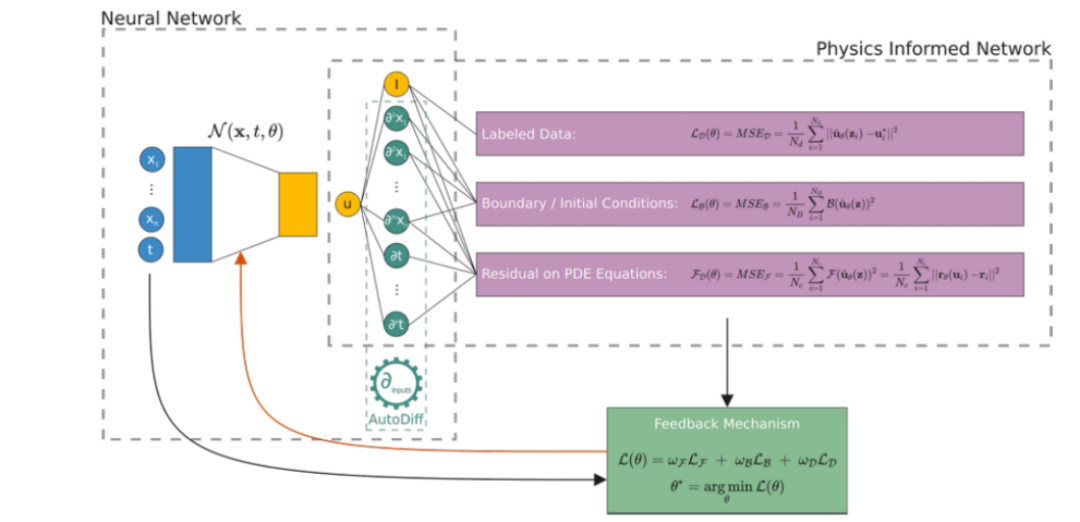
Figure 1 Schematic diagram of the composition and structure of PINN
03 · Neural network architecture
The goal of the neural network in PINN is to predict u.
Generally, a neural network can be viewed as consisting of L layers:
-
The number of network layers is L;
-
The function corresponding to the i-th layer is recorded as fi(xi, θi);
-
The entire network is used to approximate the objective function u(x).
Therefore, the network output can be expressed as:

Among them, the function composition satisfies

04 · Neural network types
4.1FFNN: Feedforward Neural Network
(Feed-forward Neural Network)
FFNN (feedforward neural network) has the following characteristics:
-
Information travels forward in one direction;
-
A common structure is MLP (Multi-Layer Perceptron, multi-layer perceptron).
Its single-level function is usually written as

Among them, is a scalar nonlinear activation function.
The entire network can be expressed as

and

Extension of FFNN - Multiple FFNN: Use multiple FFNNs for collaborative modeling to split complex problems into several parts to solve separately. For example: multiple FFNNs learn different physical processes respectively; divide the space Ω into multiple subdomains, and use one FFNN for each subdomain to solve the physical field u separately.
4.2CNN: Convolutional Neural Network
(Convolutional Neural Networks)
CNN is suitable for multidimensional data such as:
-
image;
-
voice signal.
The components of CNN include:
-
Convolution layer: The convolution kernel performs convolution on the entire input;
-
Pooling layer: reduce dimensionality.
Its functional form can be written as

Among them: α represents nonlinearity; Φ represents max-pooling; C represents the convolution operator.
4.2.1 Applications in PINN
When solving physical problems, CNN is more suitable for physical fields defined on regular and uniform grids. For situations with irregular geometric shapes and uneven grid distribution, since the adjacency relationships and actual distances at different locations are inconsistent, it is difficult for the convolution kernel of a standard CNN to naturally depict these geometric differences, so it cannot directly maintain consistent convolution operations like in image data. PhyGeoNet (physics-informed geometry-adaptive convolutional neural network) solves this problem.
PhyGeoNet maps irregular physical areas to rectangular reference areas through coordinate transformation while ensuring that the grid strictly satisfies boundary conditions.
4.2.2 Generalization: Convolutional Encoder-Decoder Network
(Convolutional Encoder-Decoder Network)
The structure includes: Encoder (the input layer is mapped to a limited number of hidden units); Decoder (the number of nodes in the output layer is the same as the input layer).
4.3RNN: Recurrent Neural Network
(Recurrent Neural Networks)
RNN can handle sequential data, so it is very suitable for processing time-related tasks, such as dynamic systems and other problems. Features of RNN include:
-
Process one input at a time and bring the hidden units from this processing into (as input) the next processing;
- Hidden units store state vectors. This vector contains information from past processed sequences.
Its functional form is written as

Among them: α is a nonlinear function; h is the hidden state vector (hidden vector state); W is the hidden-to-hidden weight; U is the input-to-hidden weight.
RNNs can handle numerical integration. Numerical integration formats such as Euler, Riemann, and Runge-Kutta can be designed as the recursive unit of RNN, thereby expressing the physical integration process as a directed calculation graph; data-driven nodes such as MLP can be added to this graph to correct the original physical model and reduce model errors.
4.3.1 Promotion: Long Short-Term Memory Network
(LSTM, Long Short-Term Memory)
The basic units of LSTM include: internal cell (internal memory unit), input gate (input gate), forget gate (forget gate), and output gate (output gate). Its function is to choose to retain or forget information in long sequence data.
In practical applications, multiple LSTM networks can be used to learn the parameters and states of the physical system, and then a tensor differentiator is used to connect these LSTM networks.
4.4
Other architectures for PINN
In addition to the above network structures, PINN can also be combined with the following models:
-
Bayesian Neural Networks (BNNs): For example, in B-PINNs, PDE constraints are used to construct the prior, and methods such as Hamiltonian Monte Carlo (HMC) and variational inference (VI) are used to estimate the posterior;
-
Generative Adversarial Networks (GANs): For example, in PI-GANs, automatic differentiation is used to encode physical laws into the generator in the form of SDEs (stochastic differential equations); and the discriminator is FFNN, which is used to compare the real input with the generator output.
05 · Introducing physical laws
The core idea of PINN is to embed physical laws into the neural network training process, and physical laws are usually represented by PDEs (partial differential equations).
The key tool is Automatic Differentiation (AD), which calculates the derivative of the network output with respect to the neural network parameters θ.
06 · Model Learning and Estimation 1 · Loss Function
The total loss function of PINN is usually written as

It contains three parts:
-
L F : Partial differential equation terms;
-
L B : Initial conditions or boundary condition items;
-
L data : Known data point verification item.
2 · Residual term LF of partial differential equation
For a single sampling point, its differential equation residual can be written as

Using the mean square error (MSE) form and randomly selecting configuration points within the definition domain, we get

Here:ωFRepresents the fidelity of the PDE model; Fidelity ↓, ωF ↓。
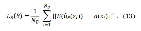
3 · Boundary/initial condition terms LB boundary terms or initial condition terms are written as
4 · Data item Ldata
The data items corresponding to the known observation data are
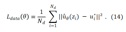
Among them: ui∗can be measured; ωdReflects the quality of the measurement.
References
Cuomo, S., Di Cola, V.S., Giampaolo, F. et al. Scientific Machine Learning Through Physics-Informed Neural Networks: Where we are and What’s Next. Journal of Scientific Computing, 92, 88 (2022). https://doi.org/10.1007/s10915-022-01939-z



Machine-translated from the Chinese original PINN: 融入物理规律的神经网络 (published 2025-04-10). WeChat original ↗