Optimal transmission theory has a history of hundreds of years, and its development has become profound and profound today. Following the development wave of artificial intelligence, especially the rise of deep learning, the optimal transmission theory has once again gained a new lease of life!
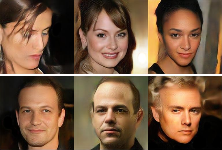
Figure 1. Realistic face images generated by a generative model constructed based on optimal transmission theory.
According to the manifold distribution law of deep learning: a type of natural data can be regarded as a probability distribution on a low-dimensional data manifold in a high-dimensional background space. The main tasks of deep learning include two, learning the manifold structure and representing the probability distribution. Deep neural networks essentially express nonlinear mappings between Euclidean spaces, so how to use mappings to represent probability distributions has become a focus of research. The optimal transmission theory is the study of mapping between probability distributions. In order to respond to the requirements of the times, we decided to teach courses on optimal transmission theory and algorithms.
During the epidemic, Lao Gu gave an online course on optimal transmission theory and algorithms to students in the Department of Computer Science and Mathematics, which is now nearing completion. The optimal transmission theory system is grand and difficult in content, making it difficult for beginners to master; the calculation of optimal transmission mapping is particularly difficult, requiring high numerical skills, and the after-school homework is very difficult. This short article aims to outline the logical clues of the course for students, and the main issues and theories covered, so that students can outline and grasp the key points, so as to be targeted and self-strengthened without being drowned in tedious details.
There are roughly three main viewpoints in optimal transport theory, and there are corresponding calculation methods: dual viewpoint, geometric viewpoint and fluid viewpoint. These perspectives complement each other and are integrated into one. The focus of our courses is on understanding theoretical systems, establishing geometric intuition, and developing practical algorithms for application in engineering practice.
dual view
French mathematician Monge proposed the Monge problem, which became the origin of optimal transmission theory.


Monge ProblemSuppose is a region in Euclidean space, and are two measures on, satisfying the condition of equal total masses. A map is said to be measure-preserving if



Abbreviated as . Given the transmission cost function, the total transmission cost of mapping is
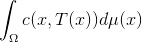
The Monge problem is to find the one with the smallest total transmission cost among all measure-guaranteed mappings:



The solution to the Monge problem is called an optimal transport map. The total cost of the optimal transmission mapping is called the Wasserstein distance between and . For example, if the transmission cost is the square of the Euclidean distance, then the corresponding Wasserstein distance is:

In deep learning, Wasserstein distance is widely used to measure the degree of dissimilarity between probability distributions. This measure is more accurate than traditional methods.
For two hundred years, the Monge problem has not been completely solved. The core reason is that the optimal transmission mapping may not exist. For example, if the source measure is concentrated on one point and the target measure is concentrated on multiple points, we need to split the source point and assign it to the target point. In this case, the optimal transmission mapping does not exist.



Kantorovich ProblemKontalovich relaxed the transmission mapping into a transmission scheme, represented by a joint probability distribution, , representing the quality of transmission from the starting point to the end point. The marginal probability of the transmission scheme is equal to and, i.e. we have



Here the projection mapping is ,. Therefore, transmission mapping becomes a special case of transmission scheme, that is, transmission mapping induces transmission scheme:

The Kontalovich problem is to find the transmission plan with the minimum cost:

The Kontalovich problem is a linear programming problem. We can use the simplex method and the ellipsoid method for optimization. However, linear programming has inherent flaws: if the optimal transmission mapping exists, then most of the variables in the optimal transmission scheme found by linear programming are wasted; at the same time, this algorithm does not take advantage of the inherent structure of the problem itself, so it is too simple and crude.
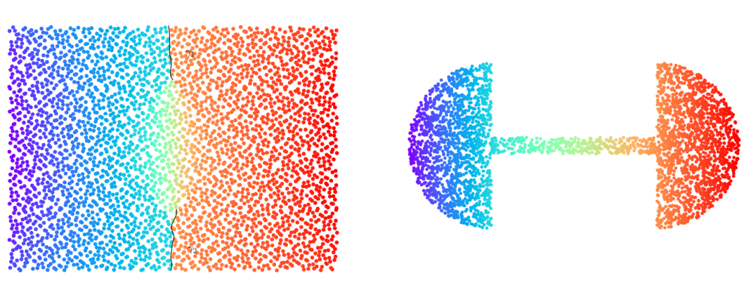
Figure 2. Optimal transmission mapping, the corresponding original image and image point are rendered with the same color.


Kantorovich Dual Problem (Kantorovich Problem)The dual form of Kontalovich's problem reveals a richer inner structure. Here, we find the sum of two functions with certain regularity, called Kontalovich's potential energy function, to maximize the following energy:


The equivalence between the primal form and the dual form of the Kontalovich problem is based on a property of the optimal transmission scheme: Cyclic Monotonocity. We take any point pair within the support set of the optimal transmission scheme:, then we have the inequality:
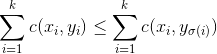

Here is an arbitrary arrangement of corner markers.
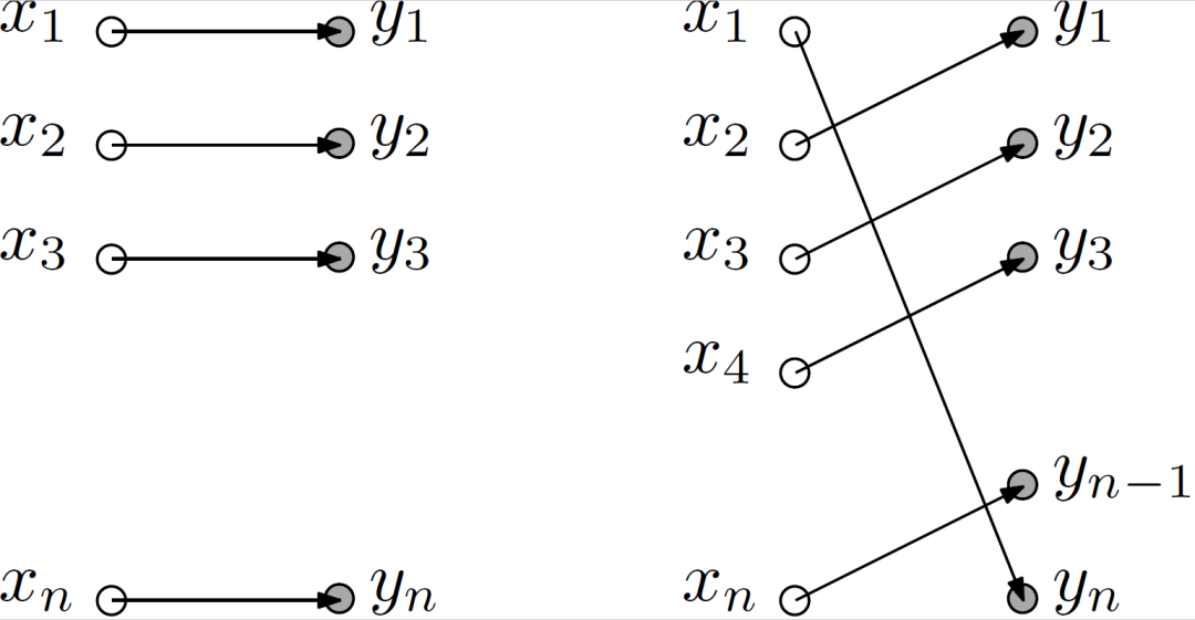
Figure 3. Cyclic Monotone.


The essence of the optimization process of dual energy is to replace the sum of the two Kontalovich potential energy functions with the c-transformation of the other party, and repeat the cycle until convergence. Here, c-transformation is a crucial concept in optimal transmission theory, defined as:


Geometrically, if we fix a point, we get a supporting surface,


The envelope of these supporting surfaces gives the c-transform.
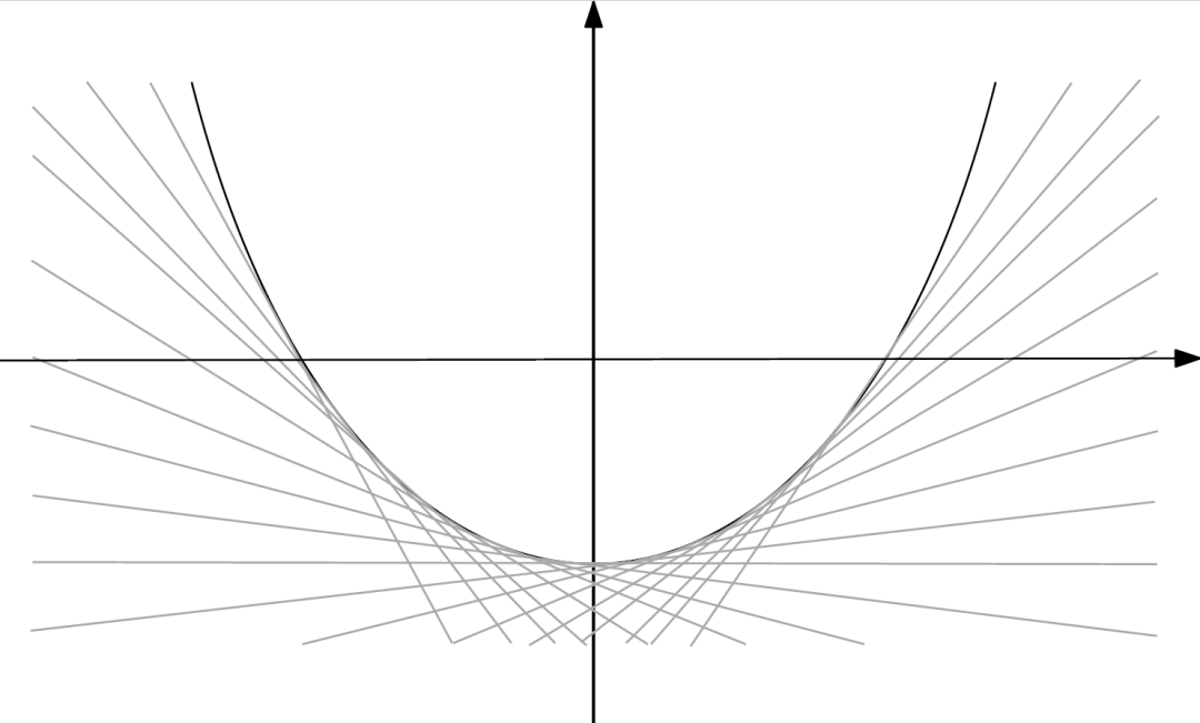
Figure 4. The support set of a convex function is a straight line, and the graph of the function is the envelope of the supporting straight line.
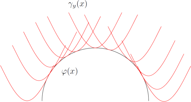
Figure 5. c-transformation.
Applying the c-transform, we get the dual problem

From here, we can derive the partial differential equations satisfied by the optimal transmission map. From the definition of c-transform, we get the points in the optimal transmission scheme support that satisfy the conditions:

If the cost function is a strictly convex function, it satisfies the form

Then the gradient mapping of the cost function is reversible, and the optimal mapping satisfies the differential equation:


Here is the optimal Kontalovich potential energy function.
Brenier problemIf the transmission cost function is the square of the Euclidean distance,
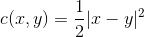
Then the optimal transfer map is the gradient map of a certain convex function:

This convex function is called the Brenier potential energy function. From the measure-preserving property of the optimal transfer mapping, we obtain that the Jacobian matrix determinant of this mapping is equal to the ratio of the probability densities of the corresponding points, thus obtaining the Monge-Ampere equation (Monge-Ampere) about the Brenier potential energy function:
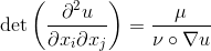

The Brenier problem is to find the Brenier potential energy function. Brenier's polar decomposition theorem asserts that any transfer map, satisfies, can be decomposed into a Brenier optimal transfer map and a voxel-preserving map.
Geometric point of view
The Monge-Ampere equation is closely linked to optimal transport theory and differential geometry. In differential geometry, the problem of replicating surfaces through Gaussian curvature ultimately boils down to partial differential equations of the Monge-Ampere type. Therefore, this class of problems can be studied either by purely geometric methods or by optimal transport theory, with these two branches providing deep insights into each other.


Minkowski Problem Given a convex surface, Gaussian mapping maps each point on the surface to the normal vector at that point, thereby mapping the Gaussian curvature of the surface onto the unit sphere to obtain a curvature function defined on the unit sphere. The Minkowski problem is to inversely solve the convex surface from the Gaussian curvature defined on the unit sphere. Historically, Minkowski proved the existence and uniqueness of solutions to low-dimensional situations, and Mr. Qiu proved the existence and uniqueness of solutions to high-dimensional situations.
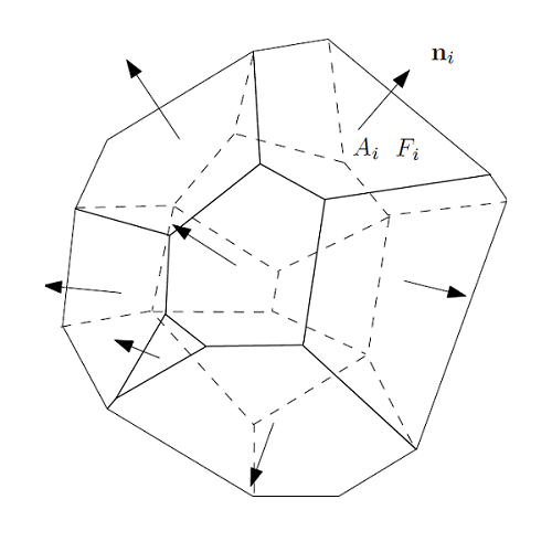
Figure 6: Minkowski problem.
The discrete formulation of the Minkowski problem is very intuitive: given a unit vector and a positive number:

Satisfy linear constraints:

Construct a convex polyhedron with the normal vector and area of each face equal to the given unit vector and a positive number, as shown in Figure 6. Minkowski can be implemented using the calculus of variations and the plane envelope algorithm.
Alexandrov Problem

Given a convex surface, its polar coordinates are expressed as



where is the polar radius function. The Gaussian curvature function of the surface is, represented by polar coordinates, we get the curvature function defined on the unit sphere, . The Alexander problem is to use the Gaussian curvature defined on the unit sphere to inversely solve the convex surface, the equivalent polar radius function. The Alexander problem is equivalent to the optimal transmission problem on the sphere, and its transmission cost is

The corresponding support surface is a plane, and it ultimately boils down to finding the envelope of the plane.
|
|
|
|
|
|
Figure 7. Solution to Alexandrov problem.
Figure 7 shows an example of solving the Alexander problem. We conformally map a monster model (upper left) onto the unit sphere (upper right), then calculate the optimal transmission mapping of the sphere (lower right), and obtain the corresponding convex surface (lower left).
Non-compact Minkowski Problem


The non-compact Minkowski problem seeks a convex function defined on a convex region. The function graph is an open convex surface such that the Gaussian curvature of the convex surface is equal to the given non-negative function .
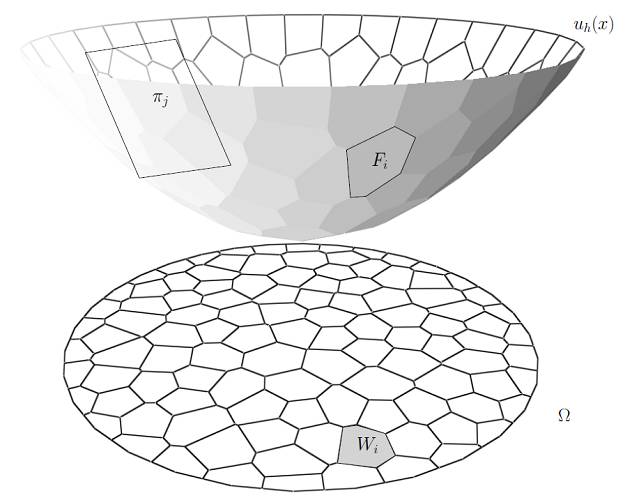
Figure 8: Non-compact Minkowski problem.

The discrete formulation of this problem is as follows: given a convex region on the plane, given a unit vector and a positive number

Satisfy linear constraints:


Construct a convex polyhedron, the normal vector of each face and the area projected to are equal to the given unit vector and a positive number, as shown in Figure 8. Alexander's theorem proves the existence and uniqueness of the solution. In essence, Alexander's theorem and Brenier's theorem are equivalent to each other and can be implemented using the variational method and the plane envelope algorithm.
|
|
|
|
|
|
Figure 9: Optimal transmission mapping calculated based on Alexandrov’s theorem.
Figure 9 shows the Brenier map calculated based on Alexandrov's theorem. We map a curved face (upper left) onto a flat disk (lower left) using Riemannian mapping. The Riemannian mapping maps the area measure (unit) of the curved surface onto a flat disk, which we call the forward measure. We use Alexandrov's theorem to calculate the Brenier map of the forward measure to the planar Lebesgue measure (the optimal transmission map under the square of the Euclidean distance), and the map image is shown in (lower right). We lay a circle packing texture image on the plane and then pull it back onto the face surface. (Top left) shows that the Riemann mapping maintains the shape of the small circle, but changes the area of the small circle; (top right) shows that the optimal transmission map changes the shape of the small circle, but maintains the area of the small circle.
|
|
|
|
|
|
Figure 10. Comparison of conformal mapping and optimal transmission mapping.
Figure 10 shows a similar calculation process to Figure 9, and we can directly compare the results of the conformal mapping and the optimal transmission mapping. Bottom left, conformal mapping brings drastic local area changes, and the density of triangulation is very different; bottom right, optimal transmission mapping maintains the area, but the shape of the triangle changes drastically. Therefore, how to design the sampling on the surface and how to construct the triangulation of the surface will have a drastic impact on the calculation of optimal transmission.
Reflector Design Problem
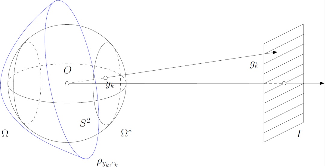
Figure 11. Reflector design issues.
|
|
|
|
|
|
Figure 12. Calculation example for mirror design.
In 1992, Mr. Qiu Chengtong proposed 100 open problems in the field of differential geometry, one of which was how to solve the reflective surface design problem. As shown in Figures 11 and 12, given an image (top left, Monge's portrait), we want to be able to design a surface, as shown in the lower row. After the light emitted from the point light source is reflected by the reflective mirror, the same image is projected on the far wall (upper right, image obtained using ray tracing method). The traditional projection equipment method uses a tiny mirror array, such as a DMD chip. Each pixel corresponds to a small mirror. The small mirror has two states, reflection and occlusion. By converting these two states at high frequency and adjusting the ratio between the two, the light intensity of each pixel can be accurately controlled. However, this method wastes a lot of light energy, and the blocked light energy is converted into heat energy. The approach here is to redistribute the incident light energy without wasting anything.
The design of this reflective optical system ultimately boils down to a spherical optimal transmission problem, which is calculated using the envelope of a convex supporting surface. Because it involves spherical geometry, we need a lot of transcendental function operations. Usually computers use Taylor expansion to approximate the operation of transcendental functions, but the accuracy cannot meet the requirements. Therefore, this type of algorithm is more difficult.
Regularity problem (Regularity)
Usually the results of calculations in the field of computer science are weak solutions, solutions in the distribution sense, or solutions in the Alexander sense, so the smoothness (regularity) of the optimal transmission mapping is not considered enough. However, some recent problems that have arisen in deep learning, such as algorithm convergence difficulties, algorithm sensitivity and vulnerability, especially mode collapse, are closely related to the regularity of optimal transmission mapping.
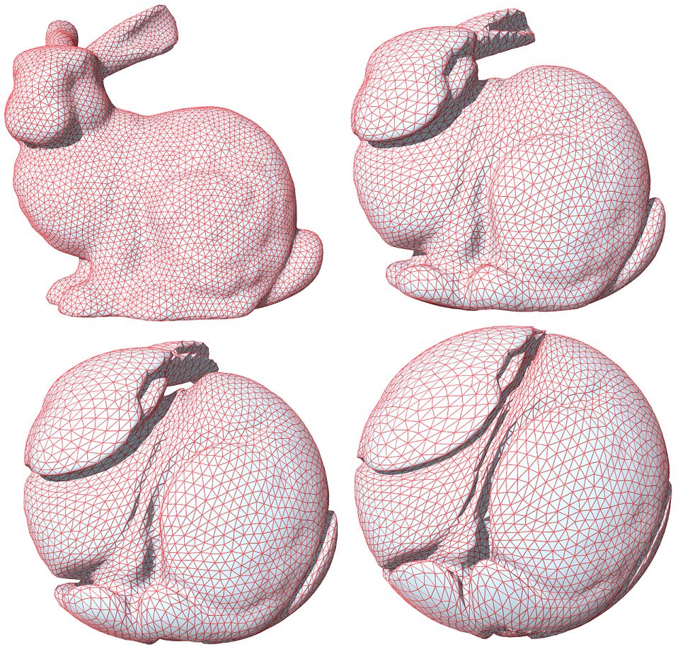
Figure 13. The optimal transmission map may be non-contiguous.


The classic Caffarelli theory reveals that the regularity of the optimal transmission mapping under distance square cost depends on many factors: the smoothness of the sum of probability density functions, the convexity and boundary smoothness of the support, and the smoothness of the cost function. The regularity problem of optimal transmission mapping under general cost functions has long been open. Villani praised Professor Wang Xujia’s research for bringing great breakthroughs. Professor Wang and his collaborators pointed out that if the fourth differential of the cost function satisfies certain conditions, then the regularity of the optimal transmission mapping is guaranteed. This condition is called the Ma-Trudinger-Wang curvature condition. Loeper gave a geometric interpretation of this curvature condition: this condition guarantees the connectivity of c-th differentials of c-convex functions.
|
|
|
|
|
|
Figure 14. The mode collapse problem that often occurs in deep learning, VAE on the upper left, WGAN on the upper right, and the model obtained by the optimal transmission theory on the bottom line improves the mode collapse.
As shown in Figure 14, we use a generative model to learn handwritten digits, and the MNIST dataset has 10 patterns. Traditional variational encoders (VAE, top left), Wasserstein GANs (top right) produce images that are indistinguishable between modes. Many times, generative models forget some patterns, a phenomenon loosely known as mode collapse.
Figure 13 gives a theoretical explanation of this phenomenon. We calculate the optimal transmission mapping (inverse mapping) between the uniform distribution inside the solid rabbit and the uniform distribution inside the solid sphere. We see that the mapping is diffeomorphic inside the entity, but the surface of the rabbit is severely wrinkled, and the mapping is no longer continuous at the wrinkles. This means that if the target region is non-convex, the transfer map is no longer continuous overall. However, deep neural networks can only express continuous mappings, and this inherent contradiction induces mode collapse.
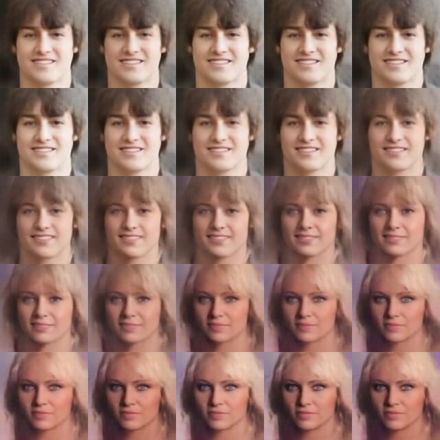
Figure 15. Edge of the face image manifold, middle row, generated samples of different colors for both eyes.
At the same time, in deep learning, the wrinkles in Figure 13 correspond to the edges of the data distribution, where the existence of samples is reasonable, but the probability of occurrence in reality is 0. For example, our training set only has black eyes or blue eyes, and the discontinuity of the optimal transmission mapping gives a generated sample with one eye black and the other blue, which is the edge of the face image manifold, as shown in Figure 15.
fluid mechanics perspective




The perspective of fluid mechanics is more consistent with physical intuition. We examine the flow of special gases in space. From a macroscopic perspective, at time, the gas density at a point in space is. From a Lagrangian perspective, the trajectory of each gas particle is a space curve. Assume that the particle trajectory is, the starting point is, and the particle speed is. If the trajectories of different particles intersect at a certain moment, a shock will appear in the flow field macroscopically. We assume that no shock wave occurs, then at that moment, the initial position of each particle is mapped to the current position, and we get the overall diffeomorphism of the whole space:





At time, the velocity vector of the particle is . At this moment, the overall velocity field of the whole space is expressed as, abbreviated as, then the diffeomorphism satisfies the ordinary differential equation:
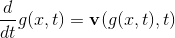


If the velocity field is given, we can get the corresponding diffeomorphism group. In other words, if the velocity field is smooth enough, no shock waves will appear in the flow field. Diffeomorphism group induced by smooth velocity field,

If the cost function is a strictly convex function, then from the Lagrangian perspective, each particle moves in a straight line at a constant speed, and its trajectory is a straight line segment with a constant speed:


Here is the optimal Kontalovich potential energy function, which is called the McCann translation.
Time Dependent Optimal Transport Problem

Given the differential cost function, defined on the velocity vector, then the entire path cost function is:
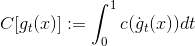


The dynamic optimal transport problem is to find a flow field connected to the sum, so that the total cost of all paths is minimized:

A sufficient condition for the equivalence of dynamic and static optimal transmission problems is that the length of the geodesic is equal to the distance between the starting point and the end point:

Assuming that the cost function is strictly convex, we look at the differential equations satisfied by the solution to the dynamic optimal transmission problem. Then by McCann translation, we get the Euler equation of the velocity field:

From the conservation of mass, we get the continuity equation for density:

Euler equations and continuity equations are valid for any strictly convex cost function, and the specific cost function information is implicit in the initial conditions. By McCann translation, the velocity of each particle is constant, so we get the initial conditions of the velocity field


Here is the optimal Kontalovich potential energy function.
Benamou-Brenier problem


Given any moment, the kinetic energy of the velocity field is





When we examine the space composed of all flow fields connecting sum, we will abbreviate it as, then






Obviously, if and only if, here, that is, the momentum has no dispersion field. The Benamou-Brenier problem finds the smallest total kinetic energy of the flow field among all:

We use the variational method to find the necessary conditions for the optimal velocity field to satisfy:



Here is any divergence-free field. According to Hodge's theorem, the optimal velocity field is "perpendicular" to any divergence-free field, so it is a gradient field, that is, there is a family of functions that satisfies . This can also be derived from McCann translation.




Tannebohm observed that under optimal transmission mapping, the vector field must be the gradient field of a certain function. The Tannenbaum algorithm first obtains a transmission mapping that satisfies, and then projects it into a divergence-free field that satisfies the Neumann boundary value condition at the boundary. The velocity field induces the flow field , thereby defining a diffeomorphism, and the transmission cost is lower than the cost of the initial mapping. In this way, we construct the flow field:
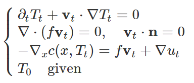


Under this flow field, the transmission cost decreases monotonically until it becomes a gradient vector field.
Benamou-Brenier introduces new energy, making the solution to the Benamou-Brenier problem a saddle point of energy, which is obtained through minimum-maximization optimization.
Algorithm Design Considerations
Compared with the classic elliptic partial differential equation, the difficulty of solving the Monge-Ampere equation is greatly increased. As shown in Figure 16, we map the human hand curved surface to a flat unit disk. During the process of calculating the conformal mapping, the triangulation of the surface does not need to be changed; during the process of calculating the optimal transmission mapping, the triangulation is constantly changing, and the final triangulation is very different from the initial triangulation. At the same time, if there is an error in the calculation process, the algorithm will crash. Therefore, how to sample the surface, how to construct the triangulation, how to maintain the convexity of the solution, and how to strictly monitor the algorithm process need to be carefully considered. In particular, current software and hardware conditions cannot support efficient high-dimensional optimal transmission mapping calculations.
|
|
|
|
|
|
|
|
|
Figure 16. Comparison of conformal mapping and optimal transmission mapping.
Summary
The three viewpoints of optimal transmission theory describe the entire theoretical edifice from different angles and provide completely different calculation methods. I hope students can master it and actively try to find practical applications in the fields of engineering and medicine. We believe that with the development of artificial intelligence, the time-honored optimal transmission theory and algorithm will follow the pace of modern times and develop further!
Machine-translated from the Chinese original “最优传输理论和算法”课程简介 (published 2020-05-03). WeChat original ↗