New book preview
The author's team compiled and summarized the classroom lecture notes and research reports on optimal transmission theory and algorithms in the past few years and published it in a book [1]. Optimal transport theory can be understood from multiple perspectives, such as linear programming and duality, convex differential geometry, Monge-Ampere partial differential equations and fluid mechanics. Each viewpoint has developed a relatively complete set of calculation methods, such as the Sinkhorn type algorithm, which is actually based on linear programming plus entropy regularization terms, or smoothing using the Nesterov method. It is currently in the field of deep learning; using Voronoi in computational geometry Diagram algorithm (C++ implementation of optimal transport geometry variation method) is based on convex differential geometry. This method can be extended to spherical geometry (C++ implementation of spherical optimal transport); the strongly nonlinear Monge-Ampère equation is iteratively approximated by the linear Poisson equation, And using fast Fourier transform to solve it is actually based on the classic theory of partial differential equations (FFT-OT: fast Fourier transform method of optimal transmission mapping); the fluid mechanics method has the strongest physical intuition, especially the optimal transmission mapping and Riemannian geometry. The last chapter of this book explains how to understand deep learning from a geometric perspective based on optimal transmission theory, explaining the intrinsic reasons for pattern collapse and new generative models. The main algorithms involved in this book are equipped with open source code and test data sets to facilitate self-study by students. The new book will be released in mid-October 2021. You can order through the following barcode:
Figure 1: Online shopping link for the new book.
I hope it can be helpful to the majority of young students. We will also further open source more related algorithms. Due to the hasty preparation and the lack of academic accomplishment of the authors, there may be loose points in the book. Readers are welcome to criticize and correct!
Basic questions
Recently, the author was invited to give a public lecture titled "Geometric Understanding of Deep Learning Based on Optimal Transfer", which is basically the last chapter of the new book. Here the author records the summary of the speech for the convenience of the audience.
Thanks for the invitation! This work is the result of collaboration with Mr. Qiu Chengtong and many mathematicians and computer scientists. At present, deep learning has achieved unprecedented success in many fields, but the theoretical understanding of deep learning is still in a relatively initial state. We try to answer the following basic questions:
-
What exactly is deep learning learning?
-
How to learn with deep learning? Did the system learn it or just remember it?
-
What is the learning quality of deep learning? Can the system learn everything? Or are you forced to forget some learning content?
what to study
Each "concept" correspondence in human vision
It refers to a family of data (point cloud) in image space. This point cloud is close to a certain low-dimensional manifold (data manifold) and satisfies a specific distribution. Therefore, computer vision is to analyze the probability distribution on this data manifold.
|
|
|
sampling
latent space
Features
encoding mapping
decode mapping
The purpose of deep learning is to learn the probability distribution on the manifold. There are two main learning tasks. One is to learn the manifold structure (explicitly or implicitly expressed as encoding and decoding mapping); the other is to learn the probability distribution (there are many ways to express probability distribution).
|
|
|
|
|
|
how to learn
Everything is approaching
Here, each neuron can only express a simple function, but multiple neurons combined to form a network can express very complex functions.
For example, the pattern recognition problem can be reduced to such a simple situation: given two closed sets and , which do not intersect each other in the topological space, according to Urysohn's lemma, there exists a continuous function and . Therefore, if the neural network can approximate this function well enough, pattern recognition can be achieved. For general manifolds, according to the Whiteny embedding theorem, the manifold can be embedded in a sufficiently high Euclidean space. Therefore, both encoding and decoding mappings exist, and the purpose of learning is to use neural networks to approximate the encoding and decoding mappings. Figure 4 shows the simplest autoencoder. There is a bottleneck layer in the middle of the network, corresponding to the hidden space. The number of neurons in the bottleneck layer is equal to the dimension of the hidden space. The network on the left side of the bottleneck layer approximates the encoding map, and the network on the right side approximates the decoding map. We densely sample on the manifold, and the loss function is designed so that the composite of encoding and decoding mappings is equal to the identity mapping. In this way, the encoding and decoding mappings are inverse mappings to each other, from the original background space to the latent space.
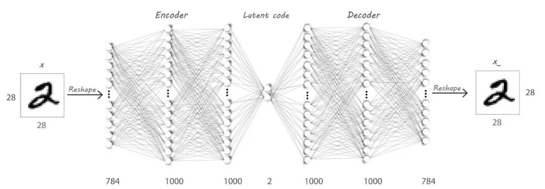
Figure 4. Autoencoder.
Figure 5 shows the learning effect. We densely sample the Maitreya Buddha surface and use an autoencoder to map the surface into the latent space, that is, encoding mapping; then decode the mapping and map the latent space back to the surface. We compare the initial data manifold with the final reconstructed surface. We see that there is not much loss of geometric information. All fingers and toes are spread out in the latent space, that is, the encoding and decoding mappings we obtain are topologically homeomorphic.
|
|
|
|
Figure 5. Manifold encoding and decoding maps learned with autoencoders.
As shown in Figure 6, we use the ReLU deep neural network, which divides both the background space and the latent space into many cells, and each cell is represented by a color. The mapping between corresponding cells is a linear mapping and can be represented by a matrix. In other words, similar to the traditional finite element method, piecewise linear functions are used to approximate the general mapping. It’s just that the finite element method uses a linear combination of basis functions to approximate any function, while the deep neural network uses a composition of piecewise linear functions to approximate it. From this, we can sayThe learning of the manifold structure is obtained by performing universal approximation through deep neural networks and performing variations in the space composed of all mappings between Euclidean spaces.However, there is no unified theory for the dynamic mechanism of learning so far. Whether the learning process converges, what the convergence rate is, and whether it converges to the global optimum all have various theoretical explanations.
|
|
|
|
Figure 6. Encoding and decoding mappings are approximated using piecewise linear mapping.
The learning of probability distributions is more complicated. We explain it with the famous generative adversarial network (GAN). According to Goodfellow's explanation, as shown in Figure 7, in the latent space
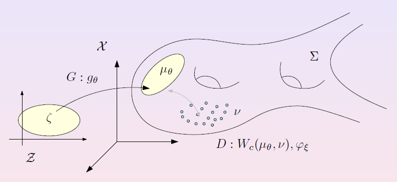
Figure 7. Theoretical explanation of GAN model.
There is a known white noise (such as Gaussian noise) in the latent space, and the generator transforms the white noise into a generated distribution on the data manifold; the training sample points on the data manifold give the real data distribution; the discriminator calculates the distance between the generated distribution and the real distribution. The discriminator and generator compete with each other and reach Nash equilibrium. The human eye cannot distinguish the generated distribution from the real distribution, and the training is terminated. Here, we see that all information about the data distribution is expressed by transformation, and the distance between two distributions is obtained by the transformation between and . So it ultimately boils down to a transformation between two probability distributions. The calculation of these transformations is based on the theory and method of optimal transmission mapping.
More broadly, the basic algorithm of statistical learning boils down to the following framework: we hope to learn a certain probability distribution, we obtain part of the information of this probability distribution through observation, express it into the expectation of a specific function, and then formulate a special energy to optimize this energy among all possible probability distributions. For example, the maximum entropy principle is to maximize the entropy of the probability distribution. The maximum likelihood method, posterior estimation, cross entropy and other algorithms are also similar. From a theoretical perspective,The learning of probability distributions boils down to optimization with restrictions on specific energy in the space composed of all distributions.. Given a data manifold, all probability distributions above form an infinite-dimensional space, which is called a Wasserstein space. The optimal transmission theory defines a Riemannian metric for Wasserstein space. With the Riemannian metric, covariant differentials can be defined, thus allowing the variational method to be implemented. Then optimization using the optimal transmission theory framework and optimization using information theory as the theory can lead to the same conclusion on classic problems (maximum entropy principle and optimal transmission).
Wasserstein space is infinite dimensional. How to define distance, geodesic, tangent vector and Riemannian metric? In other words, how to Riemannian geometrize statistics and probability distributions? This is an abstraction within the abstraction of optimal transport theory, and perhaps the most intuitive explanation comes from fluid mechanics. Suppose we have a pool (manifold) with dissolved salt in the water. The density of the salt is not uniform, giving a probability distribution. We stir the pool to move the water so that the salts are redistributed and we get another probability distribution. All possible salt distributions in the pool constitute the Wasserstein space. Given the initial distribution and the target distribution, we can design the flow field of water defined in space and time, that is, at each moment, the velocity vector at each point in the pool allows the water flow to transform the initial distribution into the target distribution. Among all possible space-time flow fields, there is only one that minimizes the total kinetic energy of the water flow (simultaneous space and time integration). This minimum total kinetic energy is defined as the distance between the initial and target distributions.Wasserstein distance. Then, this flow field has a distribution of salt at every moment, and we obtain a series of probability distributions, which constitute the link between the initial and target distributions.geodesic. At each moment, the flow field can be decomposed into a divergence-free field and a gradient field. The divergence-free field does not contribute to the change of density. Then the gradient field in the pool is defined as the probability density corresponding to that moment in the Wasserstein space.tangent vector. Then calculate the inner product of the two gradient fields bit by bit and then integrate them with respect to the entire space. In this way, we get the Wasserstein spaceRiemannian metric. If we optimize in Wasserstein space, we first calculate the variation with respect to the given energy to get a gradient field in the pool. We let the water continue to flow along this gradient field for a small time, and then get a new distribution, recalculate the variation, get a new flow field, and flow again until the resulting flow field is 0 everywhere.
Now we can answer the question above: How does deep learning learn?The deep learning system performs variation in the space composed of all mappings to learn the topological structure, and uses deep neural networks to approximate everythingCodec mapping;Optimize in Wasserstein space to learn probability distribution, which is represented by transfer map.
Learn or remember
The parameters of deep neural networks are very large, often dozens of times larger than the training samples. So a natural question is: does deep learning really learn? Or just remember it? We answer this question through a geometric interpretation of optimal transport.
|
|
|
Figure 8. Minkowski and Alexandrov problem.
Optimal transport and convex geometry have a very close affinity. As shown in Figure 8, the left frame is the famous Minkowski problem: given the normal vector and area of each face of the convex polyhedron, the shape of the convex polyhedron is determined; the right frame is the Alexandrov problem: given the normal vector of each face of the open convex polyhedron and the area projected onto the plane convex set, then the shape of the convex polyhedron is determined. The Alexandrov problem is equivalent to the optimal transmission problem under Euclidean square distance.
|
|
|
Figure 9. Brenier potential energy function.
As shown in Figure 9, according to Brenier theory, the optimal transmission map under Euclidean square distance is equal to the gradient map of a certain convex function (ie, Brenier potential energy function). The Brenier potential energy function and the Alexandrov convex polyhedron are both controlled by the Monge-Ampere equation, so they are computationally equivalent to each other. Figure 9 shows the optimal transmission mapping between the two distributions in Figure 3, and the corresponding Brenier potential energy function, as well as the inverse mapping of the optimal transmission mapping (also optimal), and its corresponding Brenier potential energy function. Through the geometric variation method (C++ implementation of the optimal transmission geometric variation method), we can accurately calculate the optimal transmission mapping. At this time, we find that the representation of the Brenier potential energy function includes all training samples and also contains new calculation variables.
From this, we can answer the above questions:This kind of deep learning remembers all training samples on the one hand, and also learns new content at the same time.
How are you studying?
Current deep learning methods are unsatisfactory, and a prominent problem is the so-calledmodel collapse. Suppose that the support set of the probability distribution we want to learn has multiple connected branches. For example, there are ten types of handwritten digits, but after learning, only six or seven are learned, and the remaining ones are forgotten; another type is pattern confusion, that is, the generated digits are a mixture of several digits and are difficult to identify. As shown in the left frame of Figure 10.
|
|
|
Figure 10. Handwritten digits generated by WGAN, compared with handwritten digits generated by AE-OT.
The problem of mode collapse can be explained by the regularity theory of optimal transmission mapping. If the support sets of the source and target distributions are both convex, the regularity of the transfer mapping is guaranteed, otherwise there may be singular points where the mapping is discontinuous. As shown in Figure 11, we calculate the optimal transmission mapping between plane probability distributions. The source distribution is a uniform distribution defined on the unit disk, and the target distribution is a uniform distribution defined on the hippocampus shape. We see that the Brenier potential energy function is continuous, but it is not differentiable everywhere. At the red curve, the Brenier potential energy function is not differentiable. The red curve is projected onto the unit disk, resulting in a black set of singular points, where the optimal transmission map is discontinued. Given a planar region, we can algorithmically determine whether there is a singular point (the "bottleneck" and "dog walking" theorem of deep learning). This creates an unavoidable essential contradiction:Deep neural networks can only approximate continuous mapping, while transmission mapping may be discontinuous at singular points, so the learning processorFailure to converge, or the image set after convergence does not match the target, resulting in model collapse。
|
|
|
|
Figure 11. Singular set of optimal transmission maps.
We can construct new generative models based on optimal transport theory to avoid mode collapse. As shown in Figure 12, we use an auto-encoder to learn the manifold structure and the optimal transfer mapping to learn the probability distribution. Deep neural networks are no longer used to approximate the transmission map, but to approximate the continuous Brenier potential energy function, or use the geometric variation method to directly calculate the Brenier potential energy function. In this way, even if the transmission map is discontinuous, it will not affect the calculation accuracy and stability.
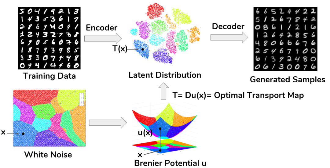
Figure 12. AE-OT generation model.
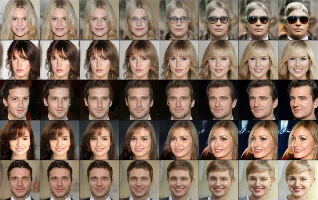
Figure 13. Edges of the face image manifold.
This generative model can accurately detect the edges of the data manifold and generate new samples at the edges. As shown in Figure 13, we used the AE-OT model to learn the manifold of a face image. We detected two boundaries of the manifold. One is a face image with brown and black eyes, and the other is a face image with blue eyes. We draw a straight line in the latent space and map it to a curve on the data manifold. Each image in Figure 13 is a point and each row is a curve. An image of a human face with one black eye and one blue eye appears on the curve. The probability of encountering such a face in real life is 0, and it is actually on the boundary of the face image manifold. The learning process is very stable, converges quickly, and does not encounter the problem of mode collapse.
Summary
Here we give a geometric explanation of deep learning: the intrinsic patterns of natural data can be expressed as probability distributions on manifolds; the main task of deep learning is to learn the structure and probability distribution of manifolds; manifold structure learning boils down to variation in the mapping space using the universal approximation properties of deep neural networks, and probability distribution learning boils down to Variations are performed in Wasserstein space; the optimal transmission theory defines the Riemannian metric for Wasserstein space, making statistical Riemannian geometry; the regularity theory of optimal transmission explains mode collapse, and the AE-OT model can be theoretically avoided, thus making the black box of deep learning partially transparent.
Please refer to [2] for details of the lecture. The new book "Theory and Calculation of Optimal Transmission" [1] can be pre-ordered by scanning the QR code. The code and data of the geometric variation method for optimal transmission mapping of the plane can be obtained from [3], which is described in detail in (C++ implementation of the optimal transmission mapping geometric variation method); the code and data of the geometric variation method of the optimal transmission mapping of the sphere can be obtained from [4], and the details are described in (C++ implementation of the optimal transmission mapping of the sphere); the algorithm that uses fast Fourier transform to speed up the solution is in (FFT-OT: Fast Fourier Transform method of the optimal transmission mapping).
【1】N. Lei, X. Gu, Theory and calculation of optimal transmission, Higher Education Press, October 2021.
【2】Na Lei, Dongsheng An, Yang Guo, Kehua Su, Shixia Liu, Zhongxuan Luo, Shing-Tung Yau and Xianfeng Gu, "Geometric Understanding of Deep Learning", Journal of Engineering, 2020.
https://doi.org/10.1016/j.eng.2019.09.010
【3】https://www3.cs.stonybrook.edu/~gu/software/OT/index.html
【4】https://www3.cs.stonybrook.edu/~gu/software/SOT/index.html
Machine-translated from the Chinese original 深度学习的几何观点 (published 2021-10-15). WeChat original ↗