On Christmas Eve 2021, Omicron is gradually declining all over the world, and it is hoped that it will disappear next year. Due to the epidemic, all teaching in 2021 will be conducted online. From late October to mid-December, the author gave a series of lectures on optimal transmission theory and algorithms online. Due to the wave of artificial intelligence, young students have shown unprecedented enthusiasm for AI theories and algorithms. We believe that the core purpose of deep learning is to learn probability distributions on manifolds. Therefore, finding the transformation between probability distributions and measuring the distance between probability distributions are indispensable operations for deep learning. How to make variations in the infinite-dimensional space composed of all probability measures is the theoretical basis of deep learning. These are the core issues in optimal transmission theory research. Therefore, the author chose this topic for in-depth elaboration.
Optimal transmission theory has a long history and is profound. Countless scientists have made outstanding contributions to it over hundreds of years, and have won Nobel Prizes and Fields Medals. Our lectures cover the outstanding work of many mathematicians such as Monge, Kantorovich, Brenier, Benamou, Minkowski, Alexandrov, Mr. Qiu Chengtong, McCann, Caffarelli, Academician Wang Xujia, Arnold, Otto, Villani, Figalli, etc., and explain them from the perspectives of classical optimal transport theory, convex differential geometry and fluid mechanics. We also cover recent developments in optimal transport theory, including Caffarrelli-McCann theory of optimal partial transport, Figalli theory, and singular set theory of optimal transport mappings. At the same time, since the majority of the audience is young students with computer science and engineering skills, we place more emphasis on the design and implementation of algorithms. On the basis of explaining the main theoretical framework, the design principles and implementation difficulties of various algorithms are explained in detail. In particular, many unique algorithms are explained, including the spherical optimal transmission algorithm designed by the author's team based on the geometric variation principle of Mr. Qiu Chengtong, the worst transmission algorithm and the optimal transmission algorithm based on fast Fourier transform. And a lot of programming homework is left to help everyone master calculation methods.
This series of lectures attracted many young students. Thousands of people attended the lectures online, which moved the author very much. The audience comes from many fields, including AI, medical imaging, computer vision, computer graphics, intelligent manufacturing, optical design, and scholars from the fields of basic mathematics and computational mathematics. There are also doctoral students in the field of mathematics who gained inspiration and inspiration through this series of lectures and completed the proof of the core theorem in their doctoral thesis, which is very gratifying! The author hopes that these theories and algorithms can be applied by the general audience in their respective fields, so that modern geometry can be more deeply and widely used in modern technology.
Below, the author sorts out the main contents of these 16 lectures and outlines them to help everyone organize the knowledge map and internalize it into their own knowledge structure. Since the author's knowledge is limited, I hope everyone can criticize and correct me.
|
|
|
| Maitreya Buddha surface | Riemann map |
|
|
|
| optimal transmission | Worst transmission |
Optimal transport theory studies how to most economically transform one probability measure to another, and it is naturally linked to convex differential geometry and fluid mechanics. In convex differential geometry, there are two measures on the convex surface, one is the area of the surface, and the other is the Gaussian curvature of the surface. The wonderful thing is that the geometry of the convex surface itself is determined by the optimal transmission mapping between these two measures. Fluid motion naturally transports fluid particles and changes the initial density into the final density. Therefore, our lectures mainly explain optimal transmission theory from three aspects: classic optimal transmission theory, convex differential geometry and fluid mechanics.
Classical optimal transmission theory
If it is differentiable, the measure-guaranteed condition is equivalent to the Jacobi equation:
Given the cost function of transmitting unit mass,Monge problemIt is to find the one with the smallest total transmission cost among all measure-guaranteed mappings:
The optimal transmission mapping transports all products from the origin to the sales location. If the sales location is not unique, the transmission mapping is generalized as a transmission scheme. Kantorovich expressed the transmission scheme as a joint probability distribution defined on , whose marginal distribution is and , is any Borel set,
Equivalently, we define the projection mapping and , and the limit of the marginal distribution can be expressed as and .Kantorovich problemExpressed as:
If we express the marginal distribution limit as a generalized Lagrange multiplier, we getKantorovich dual problem:
We introduce the concept of c-transformation:
In this way,Kantorovich dual problemImproved to:
The support set of the optimal transmission scheme satisfies
The support set of the optimal transmission scheme hascyclic monotonicity, for any points in the support set, for any arrangement, we have:
By cyclic monotonicity, we can prove that the optimal transmission scheme is equivalent to the optimal transmission mapping.
Examining the c-transform, we get
If for any fixed, there is a unique equation that satisfies the above equation, then we say that the transmission cost satisfiesdistortion condition, at this time the optimal transmission scheme (correlation) becomes the optimal transmission mapping (causality). If, here is a strongly convex function, then we have
If, we have
Substituting into Jacobi's equation, we getBrenier problem: Find a convex function that satisfies the Monge-Ampere equation:
In the c-transformation, if we are fixed, then it is a support surface, (the cost determines the support);, the envelope of the support surface gives the potential energy function, (the support envelope potential energy); define the generalized differential
The optimal transfer map , (potential energy differential map); the inverse map of the optimal transfer map is also the optimal transfer map, and is given by the generalized differential of , which is the potential energy of the inverse map, and the potential energy functions are all convex functions (map dual convex shape).
|
|
|
| Brenier potential energy function of optimal transport mapping | Legendre duality of optimal transfer potential energy function |
|
|
|
| Worst transmission Mapped Brenier potential energy function | Legendre duality of the worst transport potential energy function |
General transmission mappings can be uniquely decomposed into optimal transmission mappings and mappings that preserve the Lebesgue measure. All mappings that preserve the Lebesgue measure form a Lie group. it's famousBrenier's polar decomposition theorem。
convex geometry perspective
Consider a convex surface embedded in a Gaussian map that maps each point to its normal vector. Due to the convexity of the surface, the Gaussian map is invertible, so the surface is parameterized by a sphere. The Gaussian curvature of the surface is defined on the sphere,Minkowski problem(type II) is to find the surface from Gaussian curvature. In the discrete case, this is equivalent to giving the normal vector and area of each face of the convex polyhedron and inversely solving the convex surface. The existence of the solution to the Minkowski problem can be obtained by volume variation, and the uniqueness can be obtained by Brunn-Minkowski inequality.
If we express the convex surface in polar coordinates
Define Gaussian curvature on the unit sphere, that is, the mapping pulls the Hausdorff measure on the Gaussian sphere back to the sphere of the definition domain,Minkowski problem(Type I) is to reconstruct the convex surface based on this Gaussian curvature measure. We let the area measure and Gaussian curvature measure of the sphere be the initial and target measures, the transmission cost function is, then the optimal transmission map is, and the convex surface is the graph of the Kantorovich potential energy function.
The optimal transmission theory can be directly applied to the problem of optical lens design. Here, the incident light intensity and refracted light intensity are measurements defined on the spherical surface. The transmission cost depends on the design requirements of the optical device itself and the light conductivity coefficient of the medium. The supporting surface is a paraboloid of revolution, ellipsoid or hyperbolic surface. The potential energy function is the envelope of the supporting surface. The mapping satisfies the optical refraction law.
|
|
|
| Potential energy function of spherical optimal transmission mapping | Legendre Duality of Optimal Transfer Potential Energy on Spherical Surface |
|
|
|
| Spherical Power Diagram | Spherical Weighted Delaunay Triangulation |
If we generalize the closed surface in Minkowski (Type II) to an open surface, the Minkowski problem is generalized toAlexandrov problem. The Alexandrov problem is equivalent to the Brenier problem and both are expressed by the Monge-Ampere equation. We can use optimal transport theory to prove the existence and uniqueness of the solution, or we can use the geometric volume variation method to prove it, or the Alexandrov mapping lemma based on algebraic topology. If the Kantorovich dual problem is used to describe it, the transmission cost corresponding to the Alexandrov problem is, c-transformation is the classic Legendre transformation, the support surface is a plane, the potential energy function is equal to the upper envelope of the support plane, and its Legendre duality is the lower convex hull of the dual point of the support plane. The projection of the upper envelope on the plane is the nearest power diagram, and the projection of the convex hull is the nearest weighted Delaunay triangulation. Power diagram and Weighted Delaunay triangulation are Poincare duals to each other. From this, we see the close connection between the Alexandrov problem and classical computational geometry.
From the perspective of computational geometry, we can getWorst transmissiontheoretical framework. If we select the one with the largest total transmission cost among the metric-guaranteed mappings, we get the worst transmission mapping. In the worst-case Alexandrov problem, the potential energy function corresponds to the lower envelope of the support plane, and its Legendre dual corresponds to the upper convex hull of the dual point of the support plane. Their projections on the plane correspond to the farthest power diagram and the farthest weighted Delaunay triangulation.
|
|
|
| Medial axis of the target area | Singular set of optimal transport maps |
From the perspective of convex geometry, we can deeply understand the optimal transmission mappingsingular point set. Singular sets of optimal transfer mappings are the essential cause of pattern collapse in generative models in deep learning. From cyclic monotonicity, we obtain the slope condition of the optimal transmission map. We define the normal Frechel distance, if andNormal Frechet distanceis greater than, then there must be a singular set of optimal transmission mappings. It follows that if a plane curve has a section with a total curvature less than , and it is a convex curve, then there must be a singular point in the optimal transmission map. We further prove that the singular set of optimal transmission maps can be approximated by the Power central axis, which is equivalent to the classic central axis homotopy.
fluid mechanics perspective
Fluid mechanics has the Euler and Lagrante viewpoints. The Euler method studies the density and flow velocity of the flow field, and the Lagrange method studies the trajectory of each particle. Its initial position is and the end position is. In this way, we obtain the single-parameter differential homeomorphism family induced by the flow field,
Time-dependent optimal transmission problemis to find the flow field, and is the single-parameter differential homeomorphism family to minimize the total transmission cost (that is, the total length of all particle trajectories)
Examining the strictly convex transmission cost function, the length of the path is defined as:
From the Lagrange point of view, each particle in optimal transport moves in a straight line at a uniform speed. McCann obtained the corresponding flow field dynamics equation as:
The first equation expresses the acceleration of each particle as; the second equation is the continuity equation of mass conservation. This set of equations does not reflect the difference in transmission costs; this information is determined by the initial conditions of the velocity field.
Benamou-Brenier examined the role of the flow field (total kinetic energy),
The minimum action theorem of the flow field shows that the flow field with the smallest total kinetic energy is the solution to the time-dependent optimal transport problem, which is.
From the perspective of fluid mechanics, the optimal transport theory is connected with the infinite-dimensional Riemannian geometry theory, which defines the Riemannian metric and covariant derivatives in Wasserstein space, thus laying a theoretical foundation for the variational method in deep learning. Let us first examine the Euler equation of the incompressible flow field.
The first equation indicates that the force on the particle is equal to the negative gradient of pressure; the second equation indicates that the velocity field divergence is, that is, it is incompressible. Examining the family of single-parameter diffeomorphisms, the relationship
We obtain the Lebesgue measure-preserving mapping induced by divergence. We remember the Lie group composed of all homeomorphisms preserving the Lesbesgue measure as, given any given, we define the distance between them as:
Then the tangent vector in is the divergence-free vector field on. The first equation in the Euler equation indicates that the acceleration vector of the orbit is the gradient field on. The gradient field is perpendicular to the divergence-free field, so the acceleration of the orbit is perpendicular to the tangent space and is a geodesic. ThereforeArnold theoryIt is claimed that the Euler equation is a geodesic equation preserving the Lebesgue metric homeomorphism Lie group.
Similar,Otto theoryInterpret the Benamou-Brenier formula as the geodesic equation of Wasserstein space. Given the density field, we define the inner product in tangent space,
It can be proved that the optimal vector field must be a gradient field, that is, there is a function,
Given the tangent vector,
Their inner product is
The solution obtained by the Benamou-Brenier minimum action principle is the geodesic under the Otto Riemannian metric. The entropy flow obtained from Otto's perspective is the same as the entropy flow equation obtained from informatics.
Calculation method
We discuss almost all existing computational methods. The optimal transmission map satisfies the classic Monge-Ampere equation
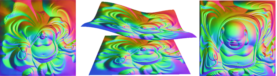
FFT-OT algorithm
Fixed point algorithm (FFT-OT) In the two-dimensional case, we note that we define the operator
Then, the Brenier potential energy function is the fixed point of the above operator and can be approximated by the iterative method. Each calculation process is equivalent to solving a Poisson equation, and the oblique boundary conditions are converted into Neumann boundary conditions. The Poisson equation can be solved using the finite difference method, accelerated by the fast Fourier transform.
continuity methodAt that time, the operator is linearized:
Here is the adjoint matrix of the Hessian matrix. We solve the Monge-Ampere equation, defining the density flow
The corresponding Brenier potential energy is, we get
order, we get
The inclination condition is transformed into a Neumann boundary condition at time , .
Tannenbaum algorithmWe first find a measure-preserving mapping, which evolves over time to gradually reduce the Monge transmission cost. Construct a differential homeomorphism, keep the measure unchanged, and combine it to reduce the transmission cost. transmission cost
The divergence component removed,
Set the velocity field. The adequacy of this algorithm for high-dimensional cases still lacks proof.
|
|
|
| Boundary conditions for volume-optimal transport mapping | Cellular decomposition of bulk-optimal transport maps |
Geometric calculus of variationsAlexandrov's theorem is equivalent to semi-discrete optimal transmission mapping. The assumed density function is absolutely continuous and is the sum of Dirac measures,
If the conditions are met, the transmission cost is the square of the Euclidean distance. For each sampling point, we construct a support plane, where the height is undetermined, and the Brenier potential energy function is the upper envelope of the support plane
Upper envelope projection results in Power Diagram
The volume of each cell is, and the transport map is, . The dual point of each support plane is, and the Legendre dual of the Brenier potential energy function is the convex hull of the dual point. The algorithm boils down to the admissible height space
, optimize convex energy
Its gradient is equal to
Hessian matrix
Here are the edges of the cell cavity and junction in the Power Diagram, which are its dual Weighted Delaunay edges.
This method can be directly generalized to other Riemannian metric cases. The implementation of the optimal transmission algorithm based on the principle of geometric variation is very challenging. The core difficulties are:
- For complex combined data structures, we introduced the simple complex half data structure and the general complex Dart data structure, and provided a library with complete functions;
- Regarding the accuracy of arithmetic calculations, traditional double-precision calculations cannot guarantee the robustness of the algorithm; theoretically perfect algorithms often collapse due to calculation errors, which requires the use of adaptive precision arithmetic operations methods.
We take plane Voronoi Diagram and Delaunay triangulation, three-dimensional Voronoi Diagram and Delaunay triangulation, plane optimal and worst transmission mapping, and spherical optimal transmission mapping as homework respectively, and provide detailed algorithm explanations and Skeleton source code to help the audience practice and master them.
Summary
We once again emphasize the formula based on the geometric point of view of optimal transmission theory to facilitate everyone's memory and application.
| cost transformation support |
| support Envelope potential energy |
| Potential energy differential mapping |
| Mapping Dual Convex
shape |
Machine-translated from the Chinese original “最优传输理论和计算”系列讲座总结 (published 2021-12-27). WeChat original ↗