Recently, many young friends have asked about the theory and calculation of optimal transmission. At that time, Mr. Qiu Chengtong taught me the relevant theory of the Monge-Ampere equation through the Minkowski problem of convex differential geometry. Therefore, the author has always understood optimal transmission and the Monge-Ampere equation through geometric pictures. Optimal transport theory has a very intuitive geometric picture and is closely consistent with classical computational geometry concepts and theories. For example, the classic Brenier theory is equivalent to the Minkowski-Alexandorff convex geometry theory (Figure 9), and the c-transformation is equivalent to the envelope in geometry. Various dualities in optimal transmission correspond to various dualities in geometry: c-transformation (Legendre transformation) corresponds to the duality of envelope and convex hull direct (Figure 3, Figure 4), forward and inverse optimal transmission transformation corresponds to the duality between Power diagram and Weighted Delaunay (Figure 2, Figure 6), optimal transmission and worst transmission correspond to the duality of upper envelope and lower envelope (Figure 2, Figure 7, Figure 8).
|
|
|
Figure 1. The Maitreya surface is mapped to the unit disk through Riemann mapping, thereby pushing the surface elements forward to the disk as the source measure for optimal transmission.
|
|
|
Most research in the field of optimal transmission focuses on solving a mapping, or Monge-Ampere equation. Here we introduce the overall geometric picture (Figure 10): that is, an infinite-dimensional functional convex space composed of all Brenier potential energy functions, and all target measures constitute an infinite-dimensional convex space. The optimal transmission mapping induces a differential homeomorphism between the two spaces. This mapping is determined point by point by the Monge-Ampere equation. We can see that under the classic semi-discrete Brenier optimal transport framework, the Brenier potential energy function space has a natural Power Digram decomposition (Power Diagram of Power Diagram), the space formed by the target measure has the corresponding Secondary Polytope structure (triangulation of triangulation), the mapping between these two functional spaces is piecewise polynomial, and the mapped Jacobian has a distinct geometric interpretation. The so-called process of solving the optimal transmission mapping can be understood as a homotopy process: given a curve segment, find its pre-image in , and by solving the inverse of the Jacobian matrix, the pre-image curve can be traced and extended point by point. This overall geometric picture provides a novel perspective for the calculation of optimal transmission problems.
In AI generation models (such as GAN models, Diffusion models), each data sample (such as a certain type of image) is regarded as a point in the high-dimensional background space, and the entire data set is regarded as a dense point cloud. This point cloud is near a certain manifold, which is the so-calleddata manifold, and the point cloud represented by the data set is regarded as aprobability distribution(probability measure). The core task of deep learning is to learn the manifold structure and the probability distribution on the manifold.encoding mappingMap the data manifold tolatent space,decode mappingMap the latent space back to the data manifold. Therefore, the topology of the data manifold is expressed by encoding and decoding maps, which are parameterized by deep neural networks. Encoding mapping maps the distribution on the data manifold to (pushed forward) the data distribution in the latent space, the so-calledHidden data distribution. We use computers to generate uniform distribution (or normal distribution) through pseudo-random numbers, that iswhite noise, and then calculate a transfer map to transform the white noise into a latent data distribution, whereby the data distribution is expressed by the transfer map, and the transfer map is also parameterized by the deep neural network. For example, in the GAN model, the generator calculates the transfer mapping from white noise to the data distribution, the discriminator calculates the optimal transfer mapping from the data distribution to the generated distribution, and the Diffusion model calculates the transfer mapping (and inverse mapping) from the data distribution to the normal distribution. It can be seen that optimal transmission lays the theoretical foundation for generative AI.
Monge-Kantorovich problem
As shown in Figures 1 and 2, given that the source region in the Euclidean space is the probability distribution of the support and has a density function; the target region is the probability distribution of the support and has a density function, a mapping is calledGuaranteed measure, if for any Borel set, there is
The measurement guarantee condition is recorded as. Given a transmission cost function, which represents the cost of transmitting unit mass from a point, the total transmission cost of the mapping is:
The famous Monge problem is to find the one with the smallest total transmission cost among all measure-guaranteed mappings:
The total transmission cost of the optimal transmission mapping is defined as the distance between and .
Kantorovich relaxes the transmission map intoTransmission scheme, that is, the joint probability distribution defined on the product space, whose marginal distribution is equal to sum, that is, , where the projection mapping is , . The Kantorovich problem translates into:
Furthermore, the Kantorovich problem is equivalent to the Kantorovich dual problem:
Here is the c-transform (a generalization of the classic Legendre transform),
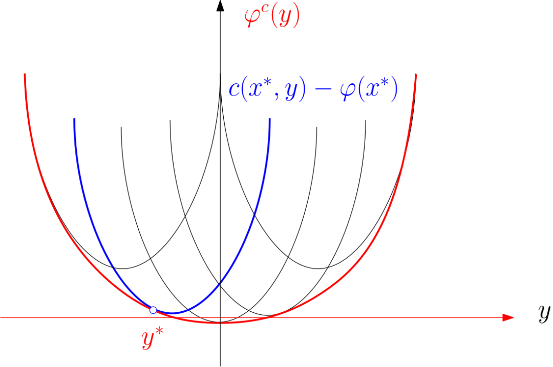
Figure 3. The c-transformation is equivalent to finding the lower envelope.
The c-transform has a distinct geometric meaning: envelope. As shown in Figure 3, when fixed and arbitrary, we define a function, the black curve in the figure; by changing it, we get a family of functions. The envelope of this family of function images is the red curve in the figure. Equivalently, we can say that each of them issupport curve. Examining the point, the red curve is tangent to the blue curve, then the optimal transmission map will be formed. We call the sum the Kantorovich potential energy function. If we can calculate the c-transform, then we can directly optimize the Kantorovich dual energy, and the potential energy function pair sequence is:
For a particular transmission cost function, we have, so the optimization terminates in finite steps. Thus, we see that geometric envelopes are a central issue in computation.
Elementary proof of optimality
We can approximate the target measure with a discrete measure (i.e., the sum of Dirac measures), assuming
The Kantorovich potential energy function defined on is denoted by , and satisfies the normalization condition
Then the Kantorovich potential energy function is equal to
induced disintegration of a cell cavity,
The energy of the dual problem can be written as:
Assume that when the energy reaches the maximum, then
That is, the volume of the cell cavity is equal to; the optimal transmission mapping is
That is, each cell cavity is mapped to a target point.
We prove below the optimality of this transport mapping. Assuming that there is another cell decomposition that satisfies the transmission mapping, then we directly compare the total transmission cost,
This proves the optimality of the transport mapping.
Brenier's theorem
If the transmission cost function is the square of the Euclidean distance, the Monge problem is expressed as
Because, therefore, the first two terms of the above equation have nothing to do with mapping. Therefore, the above Monge problem is equivalent to the following problem
At this time, the transmission cost function is. The dual problem is expressed as
At this time, the transformation is transformed into the classic Legendre transformation,
This means that the support plane is , and the gradient is .
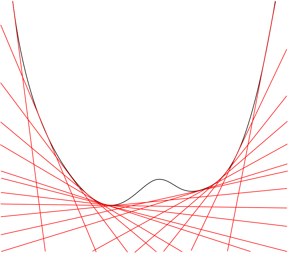
Figure 4. Convexization of a function: two Legendre transformations are equivalent to finding the upper envelope of the support plane of the function image.
As shown in Figure 4, from a geometric point of view, it is the upper envelope of all supporting planes, that is, the contained image is the smallest convex set (convex hull) containing the image. If it is a convex function, then.
Fixed, assuming that the right side reaches the maximum value, then the gradient about is zero, from which we get
At the same time, it is equal to two Legendre transformations of itself, thus it is a convex function.
|
|
|
Figure 5. Graphical illustration of Brenier's theorem.
From this, as shown in Figure 5, we get the classic Brenier theorem: at that time, the optimal transmission map is equal to the gradient map of a certain convex function, , this convex function is called the Brenier potential energy function, and at the same time, we have, , which means we get the Monge-Ampere equation:
various geometric dualities
In order to facilitate the visualization of specific concepts, we defineSemi-discrete optimal transmission Brenier problem: Let it be a convex compact set, which is a classic Lebesgue measure. The target measure is a discrete measure. The dual expression of the Brenier problem is,
Here is the Nearest Power Voronoi Diagram,
|
|
|
Figure 6. Various symmetries, summarized in the formula of optimal transmission local geometry point of view: cost transformation support, support envelope potential energy, potential energy differential mapping, mapping dual convexity.
As shown in Figure 6, we see that each target point corresponds to a support plane, Brenier potential energy function
is the upper envelope of the supporting plane family, and the projection of the upper envelope on it is the Power Diagram. Furthermore, , can be regarded as the convex hull of the point set, here it is the dual of the supporting plane. The projection of the convex hull yields the Nearest weighted Delaunay triangulation of the point set. The optimal transfer map is equal to the tangent map of the upper envelope; its inverse (generalized) map is also the optimal transfer map, and is equal to the generalized gradient map of the convex hull. Here, we see many geometric dualities, the upper envelope of the support plane family and the convex hull of the support point setDuality, nearest Power Voronoi diagram and nearest weighted Delaunay triangulationDuality, optimal transmission mapping and optimal inverse mappingDuality。
|
|
|
Figure 7. Generalization of Brenier’s theorem to worst-case transmission.
There is also a more intimate duality, optimal transmission and worst transmission.Duality, which is geometrically equivalent to the duality of the upper and lower envelopes of the support plane family. The so-called worst transmission problem is to find the one with the largest total transmission cost among all measure-guaranteed mappings:
If Brenier's theorem still holds, that is, there is a convex function, the worst transfer map is equal to the gradient map, satisfying the Monge-Ampere equation. If the target measure is a discrete measure, for each target point, we construct support planes whoselower envelope
The lower envelope is dual to the convex hull of . The farthest power Voronoi diagram obtained by the projection of the lower envelope
Its dual triangulation results in the farthest weighted Delaunay triangulation.
|
|
|
Figure 8. Upper and lower convex hulls dual lower and upper envelopes, corresponding to optimal and worst transmission.
Geometric proof of existence and uniqueness
Semi-discrete Brenier's theorem and classical convex geometryAlexandroff's theoremEquivalent. Given a convex region on the plane, it is an open convex polyhedron in , with faces, and the normal vector on each face is given, any positive number, whose sum is equal to the total area, and assuming the linear equation of the th face is , then there exists such that the projected area of the th face on is equal to . And such convex polyhedra differ from each other by one vertical translation. Therefore, we can deduce the existence and uniqueness in Brenier's theorem from Alexandroff's theorem.
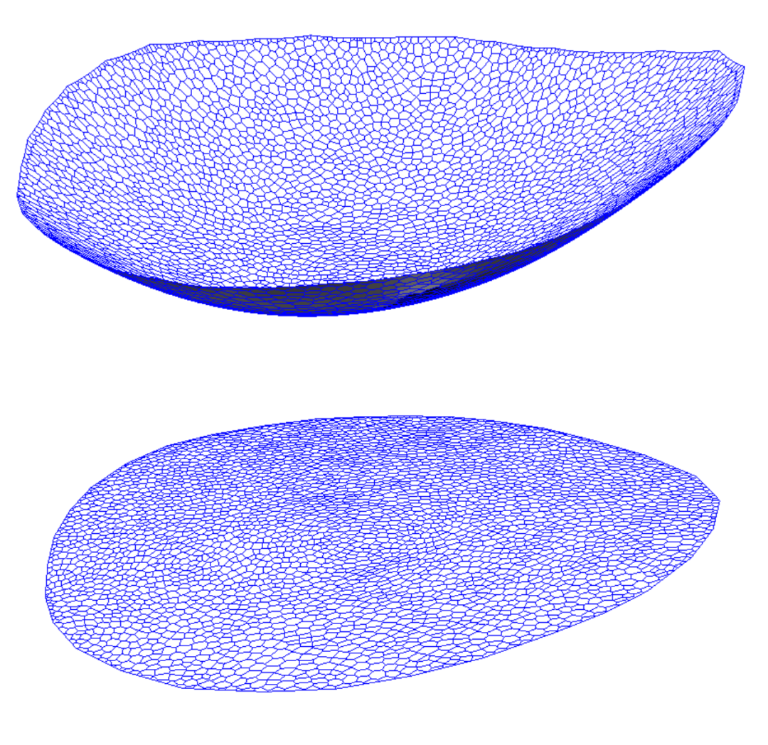
Figure 9. Alexandroff’s theorem, equivalent to Brenier’s theorem.
Below we give a simpler and more direct derivation process.
Examining semi-discrete Brenier energy:
Calculate directly and get the gradient as
Here is the volume of the Power Voronoi cell. Further calculate the Hessian matrix of energy:
The numerator here is an edge in the Power Diagram, and the denominator is the dual edge of the Weighted Delaunay triangulation. From:
We see that the Hessian matrix is strictly negative definite on the linear subspace, so the energy is strictly concave.
We define the space composed of all possible potential energy functions: that is, all those that make all Power Diagram cells non-empty,
First, it is not empty. Without loss of generality, we assume that there is a Voronoi Diagram, then
this means
Therefore it is not empty. The convexity of requires the use of Brunn-Minkowski inequality: assuming it is a convex set in Euclidean space, then
Here is the Minkowski sum of and:
Yes Lebesgue measure. If, then all Power cells, , by Brunn-Minkowski inequality,
Therefore, it is a dimensional compact convex set in .
Energy is differentiable on a compact convex set and must reach a maximum value. If , then there exists a Power cell, the partial derivative points to the interior of , so it must be an interior point of , thus,
Therefore, the solution exists. Since it is strongly concave, the maximum value is unique, so the solution is unique. This proves the existence and uniqueness of the optimal transmission mapping.
Existence and uniqueness can also be directly proved using geometric methods. The Brenier potential determines the intersection of the Alexnadroff convex polyhedron, that is, the upper envelope of the set of supporting planes with the cylinder, and then with the half-space. Examine the following optimization problem: at the intersection of the hyperplane and , find the maximum volume by using the Lagrange multiplier method:
To obtain the maximum at the interior point of , then
Because, . Assuming there are two maximum values, and the volume is the same, then according to the Brunn-Minkowski inequality, the volume is larger, thus obtaining a contradiction.
Global geometric picture of optimal transmission
From the above discussion, we see that each time the optimal transmission map is calculated, geometrically it mainly involves calculating the upper envelope of the convex hull and its dual.
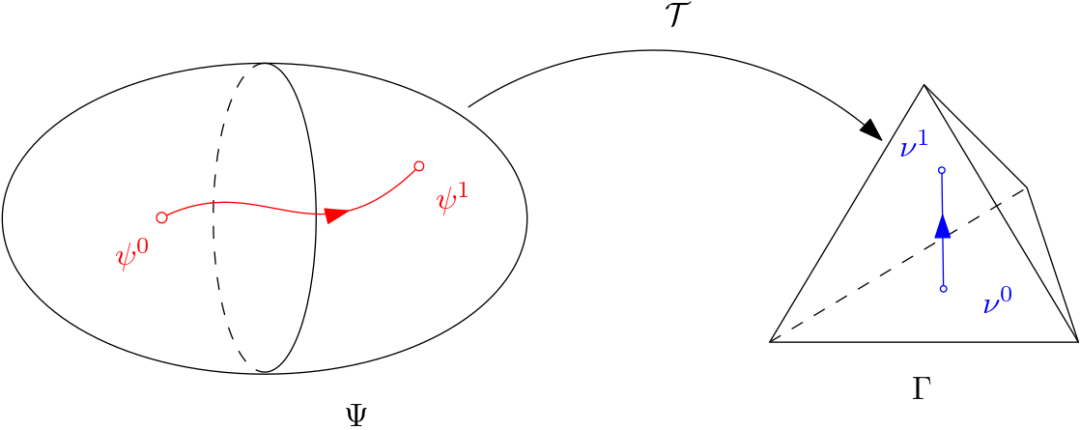
Figure 10. Global geometric perspective of optimal transmission: diffeomorphism from Brenier potential energy function space to discrete measure space. The optimal transmission problem is equivalent to the homotopy tracking problem.
We consider all optimal transmission mappings from a global perspective. All discrete Brenier potential energy functions form a convex compact set, and all corresponding discrete measures form a dimensional simplex:
Each Brenier potential energy function is mapped to a certain discrete probability measure, which is equal to the volume of the Power cell. It is the optimal transmission mapping, thus defining the overall mapping. This mapping is a diffeomorphism, and its Jacobian matrix is
Given a target measure, we hope to obtain the corresponding Brenier potential energy function. We first construct the Voronoi Digram, get , and the corresponding , and then connect and get the line segments. We want to find the original image below. The Jacobian matrix we know can be used locally for linear approximation by the continuity method (homopy method):
We can trace it step by step. Each step is equivalent to solving a Possion equation:
Here the coefficients of the Jacobian matrix are variable coefficients. The main computational difficulty is the choice of the step size, so that during the tracking process, the tracking path is always inside and returns immediately once it crosses the boundary. How to choose is the key to calculating stability. Theoretically, is a compact set, is a diffeomorphism, is a compact set, the distance to is, and the minimum characteristic root of the Hessian matrix along is, and its lower bound is, then the step size
It can ensure that no boundaries are crossed during the search process. In practical applications, we do not know the lower bounds of distance and characteristic roots in advance, so heuristics and backtracking are needed in algorithm implementation. Theoretically, the diffeomorphism here is sub-piecewise polynomial in nature, and we can compute higher-order derivatives and thus obtain accurate estimates. But so far, no one has seriously calculated these piece polynomials. The core reason is that Secondary Polytope is too complex.
Another difficulty is that the combined structure of Power Diagram and Weighted Delaunay Triangulation changes dynamically during the calculation process. A basic question is how many times does the triangulation change during each calculation? This requires the use of Gelfond's Secondary Polytope theory, which can be summarized as "triangulation of triangulations." Let be two potential energy functions. If the Weighted Delaunay triangulations they induce on are sum, then they are equivalent to each other if and are the same. Each equivalence class constitutes a cell, and the corresponding triangulation is denoted as, so our cell decomposition is:
We prove that this cell cavity decomposition is Power Diagram, that is, Power Diagram of Power Diagram.
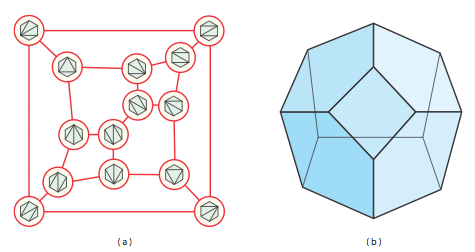
Figure 11. Gelfond's Secondary Polytope theory, that is, triangulation of triangulations. Each triangulation is abstracted into a point. The convex hull of these points expresses all triangulations. The triangulation at the boundary of the convex hull is a weighted Delaunay triangulation. Discrete and Computational Geometry, S. Devadoss and J. O'Rourke.
As shown in Figure 11, we fix the target sampling point set, , and the convex hull is recorded as . We examine all possible triangulations with vertices. We assign to each such triangulation aeigenvector(characteristic vector), the simplex is recorded as, if it is a vertex, then it is recorded as,
The secondary polytope of the point set is defined as the convex hull of all eigenvectors [2]:
If a triangulation has its eigenvector on the boundary of , then it is a Weighted Delaunay triangulation under a certain lower; if and are connected by an edge in , then they differ from each other by a Stellar transform, and in the two-dimensional case they differ from each other by an Edge swap. The dual of the convex hull is the upper envelope defined on
The Power VoronoiDiagram obtained by the projection of the upper envelope, each cell corresponds to a Weighted Delaunay triangulation, satisfying
According to Gelfand's secondary polytope theory [2], the number of all possible Weighted Delaunay Triangulation is , and the diameter is , which gives the number of changes in the triangulation combination structure during the calculation of the optimal transmission map. We see Guelfond's secondary polytope (triangulation of triangulation) is dual to the Power Diagram of Brenier potential energy function space (Power Diagram of Power Diagram); according to Brenier's theorem, we obtain the mapping, which is the optimal transmission mapping; for specific details, please refer to [1]. At present, there is almost no research on the algorithm of this two-dimensional power diagram. We expect that research in this area can make breakthroughs.
Currently, in the fields of AI and computer science, people only calculate the weak solution of the optimal transmission mapping, and there is little discussion on the regularity of the solution. The regularity theory of the Monge-Ampere equation requires more profound and subtle geometric insights. In the future, when computer science develops further, the geometric picture of optimal transmission regularity theory will penetrate.
Summary
Here, we summarize the geometric perspectives of optimal transport theory, including local and global perspectives. From a local point of view, the formula for solving an optimal transmission problem is "cost transformation support, support envelope potential energy, potential energy differential mapping, mapping dual convex shape". This involves a large number of symmetries, which can be understood from both analytical and geometric perspectives. The Legendre transformation corresponds to the duality of the upper envelope and the convex hull, and the forward and inverse optimal transmission corresponds to Power Diagram and Weighted The duality of Delaunay, the duality of the optimal and worst transmission corresponding to the upper envelope and the lower envelope, the universal c-transform corresponding to the surface family envelope, etc.
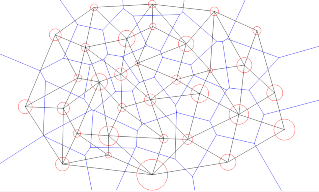
Figure 12. The duality of Power Voronoi Diagram and Weighted Delaunay Triangulation naturally appears in the local geometric point of view and the global geometric point of view of optimal transmission.
On the whole, the optimal transfer gives a differential homeomorphism between the space composed of all Brenier potential energy functions and the space composed of all measures. Its Jacobian matrix is given by the ratio of the Power Voronoi side length and the Weighted Delaunay side length. Furthermore, this differential homeomorphism is a piecewise polynomial; the convex hull of all possible Weighted Delaunay triangulation eigenvectors constitutes the Gelfond Secondary Polytope, that is, alltriangulation of triangulation, whose dual is allPower Diagram of Power Diagram, that is, the Power Diagram of the space composed of all potential energy functions, and each cell corresponds to a triangulation. Compared with the local geometric point of view, the global geometric point of view has not been widely explored and has broad research prospects.
Acknowledgments
Thanks to Academician Qiu Chengtong for his teaching, Professor Luo Feng, Professor Wang Xujia, Professor Zhao Guohui and other mathematicians, whose in-depth discussions inspired our work [1]; thanks to all collaborators and classmates. Cover credit: @GIORDANOPHOTOGRAPHY ON INSTAGRAM
【1】Na Lei, Wei Chen*, Zhongxuan Luo, Hang Si, Xianfeng Gu. Secondary Polytope and Secondary Power Diagram. Computational Mathematics and Mathematical Physics, 2019,59(12):1965-1981.
【2】M. Gel’fand, M.M. Kapranov, and A.V. Zelevinsky. Discriminants, Resultants, and Multidi-mensional Determinants. Birkhauser, 1994.
Machine-translated from the Chinese original 最优传输理论的全局几何观点 (published 2023-11-06). WeChat original ↗