When EE starts in the spring of 2024, many young people come to visit the author to discuss future research directions; many friends from academia and industry also discuss technology development trends with the author. Everyone is very interested in IGA (isogeometric anylasis) in the CAD/CAE field. Isogeometric analysis is currently regarded as the most revolutionary breakthrough in the field of CAE, but it has inherent difficulties. The author's team believes that the Riemann-Roch theorem in complex geometry will play a decisive role in solving the core difficulties in isogeometric analysis. Riemann-Roch has long been regarded as an aesthetic representative in abstract mathematics. We are delighted to find that due to the rise of isogeometric analysis, this purely elegant theory is expected to enter the field of engineering, thereby achieving the unification of aesthetic and practical values. Here the author will briefly explain the intrinsic relationship between the two and explore the potential impact of Riemann-Roch theory on the development of the CAD/CAE field.
The Blooming Theory of CAD
Computer Aided Design (CAD) originated in the 1970s. Its core task is to use computers to express geometric surfaces and help engineering designers design various industrial products. The Bezier Spline was first invented by Bezier of the French Renault Automobile Company. Later, it was popularized as B-Spline curves and surfaces. Currently, non-uniform rational B-spline surfaces have become the industry standard. In the 2000s, Dr. Tom Sederberg further promoted them as T-spline surfaces.
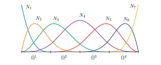
Figure 1. B-spline basis functions.
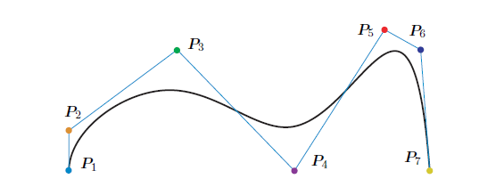
Figure 2. B-spline curve.
The classic definition of B-spline curve is as follows: given the node vector on the parameter straight line, the B-spline curve with order n control vertices is defined as
Here are the control points, called spline basis functions. All spline basis functions constitute unit decomposition, that is, for the desired parameters,
At the same time, the support of each basis function is a compact set. A B-spline can be thought of as some kind of weighted average of control points. Here the B-spline basis function is defined recursively, and the recursive basis is
The recursive relationship is
Figure 1 shows the basis functions of a B-spline, and Figure 2 shows the B-spline curve. A more modern approach is the so-called "Blossom" theory. Given a unit-order polynomial
The existence of an elemental, symmetric, multi-affine polynomial is called its bloom, or polar form.
satisfy
Symmetry here means that any permutation of the independent variables does not change the polynomial,
multi-affine means
The blooming of an order B-spline is that, given the node vector, then the control vertex is actually blooming
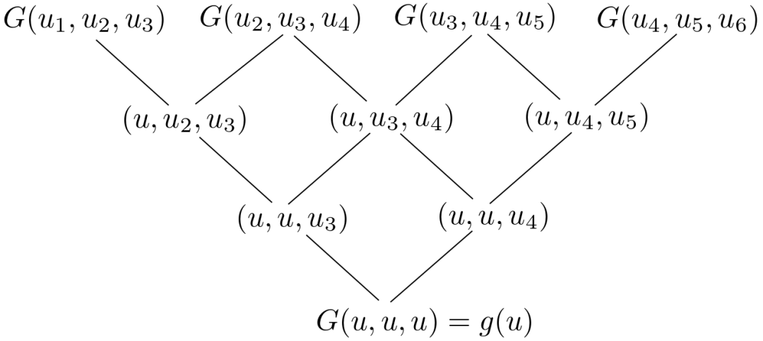
Figure 3. de Boor evaluation algorithm for B-splines.
The de Boor algorithm for evaluating B-splines is a recursive algorithm based on various properties of flowering, as shown in Figure 3, where the first step
The tensor product of spline curves gives the spline surface:
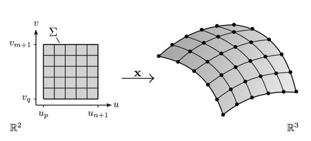
Figure 4 shows a spline surface. We see that the node vectors in the and directions form a quadrilateral mesh.
In order to express more complex shapes, such as standard circles, people generalize polynomial spline curves and surfaces to rational spline curves and surfaces. The most common one is NURBS (non-uniform rational B-Spline surface). Each control point adds a weight factor.
In practical applications, if the surface has many geometric details, we often need to refine the spline surface. In this case, nodes and control points need to be added while keeping the shape of the curve and surface unchanged.
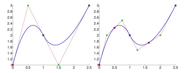
Figure 5. B-spline adding nodes.
We can understand the refinement node from a blooming perspective. Assuming that the initial node vector is, we add new nodes between and to get a new node vector.
From the new node vector, we get the newly added control point,
Because the bloom has not changed, the B-spline shape has not changed. Figure 5 shows the nodal refinement of the B-splines.
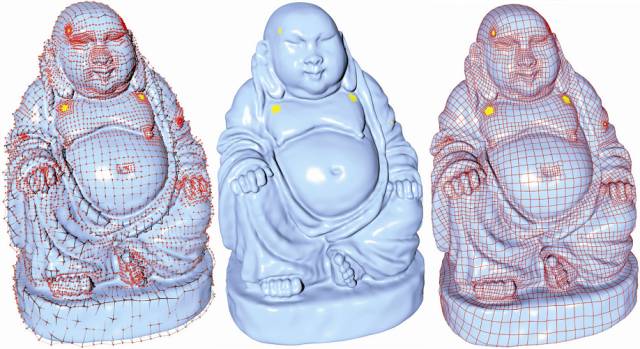
Figure 6. T-spline surface.
On traditional NURBS, node refinement is global, that is, whenever we add nodes in one place, we need to keep the nodes forming a quadrilateral grid, so we need to add nodes along a curve on the surface. Many times, we only want to change the node structure of NURBS locally and do not want to affect the global situation. The T-spline proposed by Sederberg is to solve this contradiction. The T-spline allows users to add nodes locally, and all nodes constitute the T-grid structure on the surface, as shown in Figure 6.
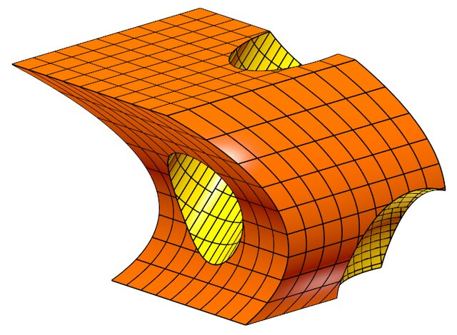
Figure 7. Clipping spline.
Figure 7 shows the geometric model constructed with trimmed-spline surfaces. The so-called clipping spline surface is to cut out some holes on the traditional spline surface patch, and the edges of these holes are described by spline curves in the parameter domain. CAD models in engineering applications widely use clipping splines, but clipping splines cannot be applied to isogeometric analysis, which is one of the obstacles to the direct promotion of isogeometric analysis.
CAE’s Galerkin method
Almost all physical laws are described by partial differential equations. Numerical simulation of various physical phenomena is equivalent to solving various partial differential equations on geometric models. The core of CAE (Computer Aided Engineering) is to perform multi-physics numerical simulation on geometry. The Finite Element Method (Finite Element Method) developed by applied mathematicians such as Courant in the 1940s is the most common method in CAE. Chinese mathematician Feng Kang also independently laid the theoretical foundation of finite element. Let's take Poisson's equation as an example to introduce the most commonly used Galerkin method. Examine the heat conduction equation in Euclidean space: find the second-order smooth function, , which satisfies the Dirichlet boundary condition:
First, we transform the strong form of the partial differential equation into the weak form, let be a smooth function with compact support, which we call the test function, multiply both sides of the Poisson equation, and then integrate, we get
Integrate by parts and test the function on the boundary,
This leads to the weak form of the partial differential equation. For any test function,
Define a bilinear functional
and linear functionals
The weak form of Poisson's equation is expressed as the search function, ,
The weak form only requires that the unknown function has first-order derivatives, while the strong solution of Poisson's equation requires second-order differentiability, and the weak solution reduces the smoothness requirement.
The Galerkin method uses a finite-dimensional function space to approximate the original function space.
Here are the basis functions of a discrete function space with compact support. We use linear combinations of basis functions to approximate the unknown function
These basis functions can also be used as test functions to obtain linear equations,
This gives us a system of linear equations:
What is called here is the stiffness matrix, which is symmetric and positive definite and is the control point of the unknown function. The linear elliptic Poisson equation is thus transformed into a system of linear equations.
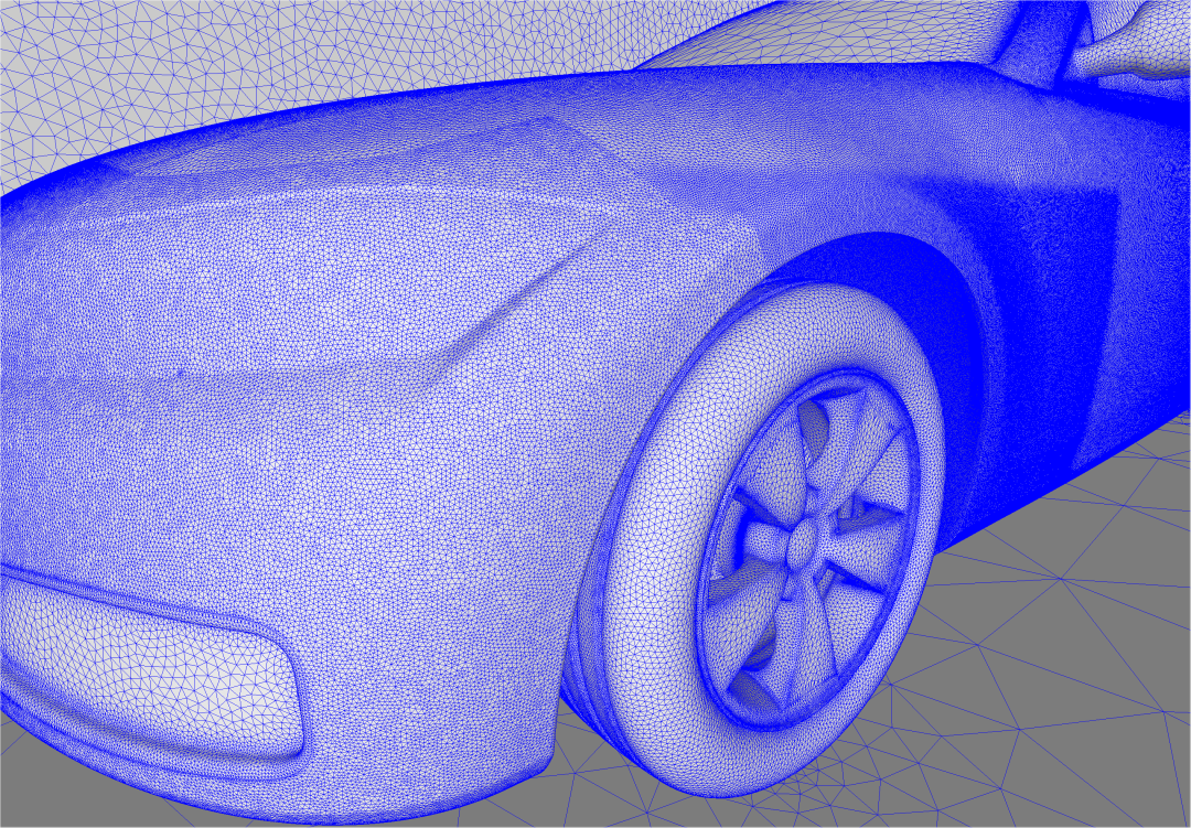
Figure 7. The traditional finite element method is based on triangulation.
As shown in Figure 7, the traditional finite element method is to triangulate the geometry and then establish basis functions on the triangulation. For example, we have a tetrahedral mesh, and considering one of the tetrahedrons, whose vertices are, we defineCenter of gravity coordinates, suppose, then
Then the basis function corresponding to the vertex is limited to, which is
Since the support of each basis function is defined on adjacent tetrahedrons, the stiffness matrix itself is sparse. In the finite element algorithm, we calculate the stiffness matrix on each element (tetrahedron) and then assemble it into the overall stiffness matrix.
We see that in the traditional CAD industry, all geometries are represented as NURBS surfaces; in the traditional CAE industry, geometries are represented as meshes, often triangulations. Converting CAD models into triangulations is the most time-consuming and computationally resource-intensive step in the entire digital simulation process, generally accounting for more than all computing time. At the same time, grid discretization will bring geometric errors, which is a key factor affecting the accuracy of simulation problems.
IGA’s Thoughts and Challenges
In 2005, Dr. Tom Hughes proposed the idea of isogeometric analysis. The core is to use a unified spline language to express geometric shapes and physical fields: use planar NURBS parametric surfaces or volume NURBS parametric volumes as the calculation domain, and the calculation unit is the surface unit or volume unit corresponding to the node interval; use the NURBS basis function as the basis function (shape function) of the physical field, and use the physical mathematical components of the control vertices as unknown variables. In this way, shape geometry and analysis geometry are in the same spline space, avoiding data exchange; simulation calculations are performed on precise CAD geometry to avoid geometric discrete errors; with the same degree of freedom, higher calculation accuracy is achieved, or with the same accuracy, fewer degrees of freedom are required. At the same time, the physics simulation maintains smoothness. From an engineering perspective, isogeometric analysis is compatible with traditional finite element methods and can be integrated into existing finite element environments.
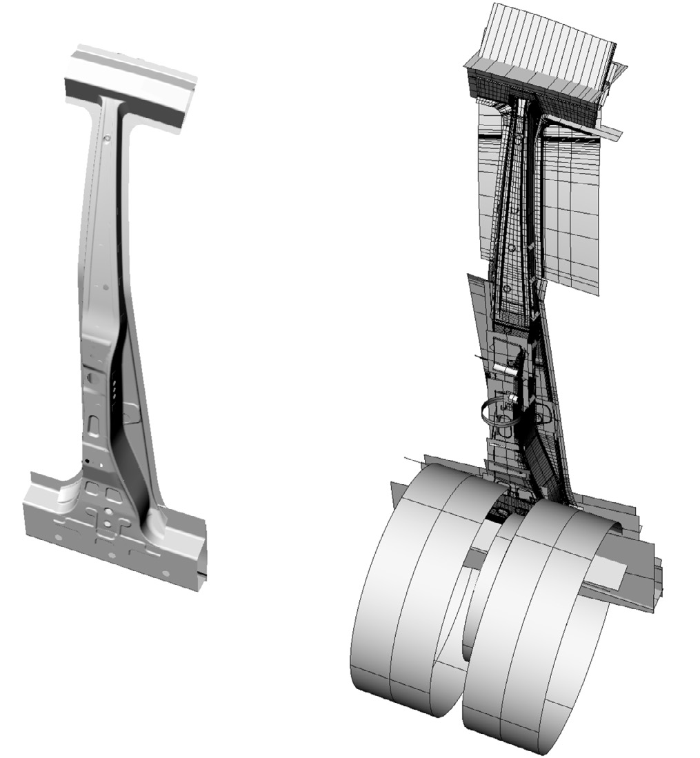
Figure 8. The traditional automobile B-pillar model uses a large number of clipped surfaces and cannot be applied to isogeometric analysis.
Although isogeometric analysis has many advantages that traditional methods cannot match, isogeometric analysis has not been widely adopted by the industry. The core is that the spline surfaces in the traditional CAD industry cannot meet the requirements of isogeometric analysis. Traditional NURBS uses a large number of clipping splines. The clipping splines cannot be decomposed into regular units and need to be reconstructed; traditional NURBS lacks watertightness and has a large number of gaps, so there are many fragmented splines to make up for the gaps, which need to be merged into whole splines. The most fatal problem is that the traditional CAD model only expresses the boundary surface of the geometry, while isogeometric analysis requires the interior of the entire entity to be expressed as splines.
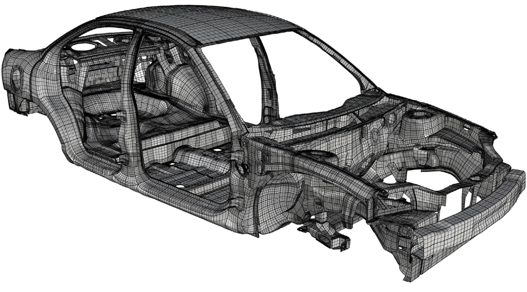
Figure 9. Traditional CAD models need to be converted into spline surfaces that satisfy isogeometric analysis.
Therefore, converting traditional CAD models into splines that meet the requirements of isogeometric analysis requires the generation of overall structured quadrilateral meshes for surfaces and the generation of overall structured hexahedral meshes for solids. These two problems are open problems in the fields of traditional CAD and CAE, and the required mathematical theory is different from the theoretical basis of traditional CAD/CAE. The basis of traditional CAE theory lies in classical analytical theories such as linear elliptic partial differential equation theory, Sobolev space theory, and variational principles; traditional CAD theory lies in polynomial algebra, such as Bayou's theorem, Grobner basis, Nord's theory, and the ideal theory of polynomial rings; while the overall spline construction requires the affine structure theory of manifolds, etc.
The node mesh of the global NURBS representation (or T-spline representation) of the surface is the global quadrilateral mesh (or T-grid) on the surface. The two families of NURBS isoparametric curves will produce an overall quadrilateral mesh of the surface. In general, the two families of isoparametric curves should be perpendicular to each other at the intersection points, and each quadrilateral should be close to a planar square (different sizes). Vertices on the mesh whose topological degree is not equal to 4 are called singular points. Well, finding the governing equations satisfied by singular points has been one of the basic problems in the field of engineering for a long time. The vigorous development of isogeometric analysis makes the solution of this problem more urgent.
Riemann-Roch theorem
The breakthrough in this problem is based on Riemann surface theory (algebraic curve theory). In complex analysis, a complex-valued function is said to be analytic if, for any point, there exists a neighborhood in which the function has a Laurent expansion:
The order of the function is recorded as, if , then it is the pole, if then it is the zero point. An analytic function is said to be holomorphic, or meromorphic if it has poles. If the surface exists an open cover, each open set has local complex coordinates, and any coordinate transformation function
are all holomorphic, and their inverse mapping is also holomorphic, then the atlas is called a conformal atlas, and the surface is called a Riemann surface. All surfaces in the physical world are orientable surfaces with Riemannian metrics, and it can be proven that they are all Riemannian surfaces.
Concepts of complex analysis such as analytic functions can be directly extended to the Riemann surface, which is called a holomorphic (meromorphic) function. If it is restricted to each local coordinate, it is holomorphic (meromorphic). The logarithm of the module of a holomorphic function is a harmonic function, and the harmonic function satisfies the mean value theorem, that is, the extreme value of the function is not taken at the interior point. Therefore, if the Riemann surface is compact, then the holomorphic function must be constant. But the meromorphic functions on the compact Riemann surface are very rich. The sum, difference, product and quotient of any two meromorphic functions are still meromorphic functions, so all meromorphic functions on a Riemann surface constitute a domain. If the fields of meromorphic functions on two Riemann surfaces are algebraically isomorphic, then the two Riemann surfaces are isomorphic as complex manifolds. Holomorphic differentials and meromorphic differentials can also be generalized to the Riemann surface, let it be a complex differential form, if on each local coordinate, , on other local coordinates
If it is holomorphic (meromorphic), it is called a holomorphic (meromorphic) differential. The spaces of all holomorphic differentials are denoted by , and the spaces of all meromorphic differentials are denoted by .
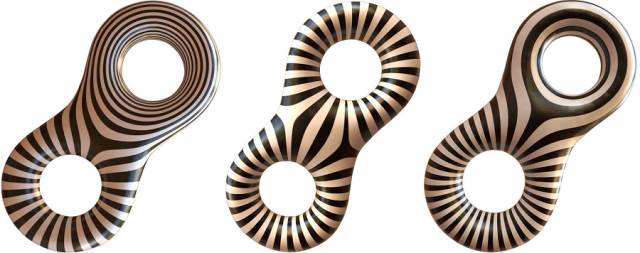
Figure 10. Holomorphic quadratic differential on the Riemann surface.
The basis of the fundamental group whose genus is the Riemann surface is written as, and the basis of all holomorphic differential forms is, we define a vector
From the Riemannian bilinear relationship, we get the generation of a non-degenerate lattice, and the Jacobi variety of the Riemannian surface is defined as
The Abel-Jacobi mapping is defined as
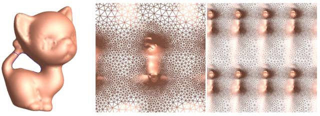
Figure 11. Abel-Jacobi map of the Riemannian surface with genus one.
The divisor on the Riemann surface is an integer linear combination of a finite number of discrete points, and the degree of the divisor is defined as. Given a meromorphic function, its divisor is called the principal divisor and is defined as
Abel's theorem asserts that a divisor is a principal divisor if and only if
Given a divisor, we define a linear space: the space composed of meromorphic functions whose divisors are greater than or equal to
Similarly, the space consists of meromorphic differentials with all divisors greater than or equal to
Riemann-Roch theoremAssert the relationship between the difference in the dimensions of these two linear spaces and the topology of the Riemannian surfaces:
Abel's theorem determines whether there is a meromorphic function with a given divisor; the Riemann-Roche theorem (RR theorem) infers the number of dimensions of the meromorphic function space that satisfies greater than or equal to.
The inner connection between IGA and RR
Isogeometric analysis requires a globally watertight spline representation, which boils down to a globally structured quadrilateral mesh of the surface. The key to constructing a quadrilateral mesh is to determine the location and indicators of singular points. For decades, the determination of singularities relied heavily on the manual input of engineers. Finding the governing equation of singular points is a basic theoretical problem.
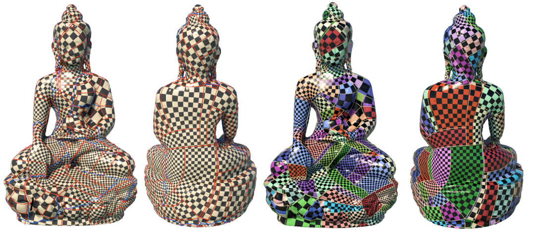
Figure 12. The singular points of the structured quadrilateral mesh (T-grid) of the curved surface satisfy Abel’s theorem.
Suppose it is a surface in the physical world with a Riemannian metric induced by the Euclidean metric. Assuming the quadrilateral grid (or T-grid) above, the two families of grid lines are perpendicular to each other, and each face is close to a square. We establish a local complex coordinate for each surface and establish a meromorphic differential locally, then we can prove
is the meromorphic fourth differential defined as a whole. We arbitrarily choose a holomorphic differential form, then
is a meromorphic function whose divisor is the principal divisor and satisfies Abel’s theorem
This givesGoverning Equations of Singular Points of Surface Structured Mesh, here the mesh includes quadrilateral mesh and T-grid. If the singular point configuration given by the user does not satisfy Abel's theorem, the algorithm can optimize the position of the singular point to satisfy the theorem, then apply Ricci flow to calculate the straightness metric, concentrate all curvatures on the singular points, and then construct an overall structured grid on the straightness metric.
Furthermore, if the location and index of some singular points are given, denoted as We can also optimize in this solution space and select the optimal mesh that meets the engineering requirements to provide qualified spline surfaces for isogeometric analysis.
The Riemann-Roche theorem is the central theorem of Riemann surface theory (algebraic curves). It is essentially an index theorem that connects analysis (meromorphic functions, meromorphic differential spaces) and topology (genus). From a modern point of view, given the divisor, we can construct a holopure line bundle. The local meromorphic cross-section of this line bundle constitutes the sheaf. The obstacle for the local cross-section to merge into the global cross-section can be described by the Cech cohomology of the sheaf. The staggered sum of the dimensions of the Cech cohomology group is the Euler characteristic number. The Riemann-Rohe theorem essentially describes the Euler characteristic number of the holopure line bundle.
Summary
Isogeometric analysis unifies data representation in the CAD and CAE fields, reduces calculation errors, and improves efficiency. It is the most revolutionary invention in the CAD/CAE field in recent years. However, traditional CAD models cannot meet the requirements of isogeometric analysis. In order to meet the requirements of isogeometric analysis, structured quadrilateral meshes and hexahedral meshes have become bottlenecks in technological development. The theoretical basis of surface structured grids is the Abelian-Jacobian theory and the Riemann-Roch theory of algebraic curves.
The Riemann-Roche theorem has always been a pure and elegant representative of abstract mathematics. Unexpectedly, this theorem actually provides a powerful computing tool for isogeometric analysis in the CAD/CAE field, describing the dimensions of the solution space of a structured grid (T-grid) that meets specific conditions. We sincerely hope that this simple and beautiful theorem can shine in the industrial field and truly achieve a high degree of harmony and unity of aesthetic value and practical value.
Machine-translated from the Chinese original 等几何分析与黎曼-罗赫定理 (published 2024-03-28). WeChat original ↗