Mr. Qiu Chengtong believes that "mathematics plays an important role in the fields of artificial intelligence and big data. It is not only the core foundation of algorithms and technologies, but also the key to understanding the deep meaning of big data. Many mathematical theories that were once considered abstract have now become concrete tools to solve core problems in science, technology, economy and society." Mr. Qiu's assertion about the foundation of AI now points the way for large language models that are mired in "illusion". When AI misjudges the cough, fever, and dyspnea of pneumonia as colds during medical diagnosis, and casually recommends "drink more water and rest", the patient may miss the best treatment window; when the AI-generated legal document submitted by the lawyer suddenly appears "Article 12 of the Civil Code" 34", not only will they face court fines, but they will also waste already strained judicial resources; when researchers follow the reference documents of "Quantum Noodle Theory" fabricated by the model, precious academic energy is being led astray.
These seemingly isolated hallucination phenomena actually expose the underlying flaws of the generative model: its knowledge space is like a manifold with "singular points" in differential geometry - erroneous information that violates logical facts is hidden in abnormal areas with sudden changes in curvature, and the process of the model generating content is like the path deviation that falls into these traps when there is a lack of rigorous navigation. When the probabilistic maze of AI meets the logical beacon of differential geometry, can the geometric analysis founded by Mr. Qiu become a mathematical compass for calibrating cognitive biases? The dialogue between cross-domain mathematics and artificial intelligence may be pregnant with fundamental breakthroughs that eliminate the illusion of AI.
|
|
|
Figure 1. Sora produces hallucinations in short videos.
imagination and hallucinations
The so-called "AI hallucination" refers to the false, inaccurate or inconsistent information output by the AI model. This information usually seems convincing, but is actually wrong or inconsistent with the real world (violating the laws of physics, biological laws, etc.). For example, in Figure 1, the short video generated by Sora looks very realistic, but there are many absurdities. For example, in the "Puppies on the Lawn" video, there are three puppies and four puppies in one moment, which obviously violates the laws of biology and physics; in the "Red Wine in a Glass" video, the red wine is spilled before the glass is poured, which violates fluid mechanics; the "Four-Legged Ant" video violates the laws of biology, etc. Figure 2 is a common illusion in Vincentian diagrams. When we give the prompt word "rabbit and tortoise", the model generates a creature with a tortoise body and a hare head. This is a common illusion in token-based generative models. On the contrary, the so-called "imagination" refers to the real, accurate and factual information output by the AI model, which satisfies all physical laws, biological laws and other natural laws. These generated data may not completely coincide with the training samples, but they conform to the statistical laws of the training set.

Figure 2. The illusion of Vincentian diagram, rabbit and turtle.
manifold distribution rule
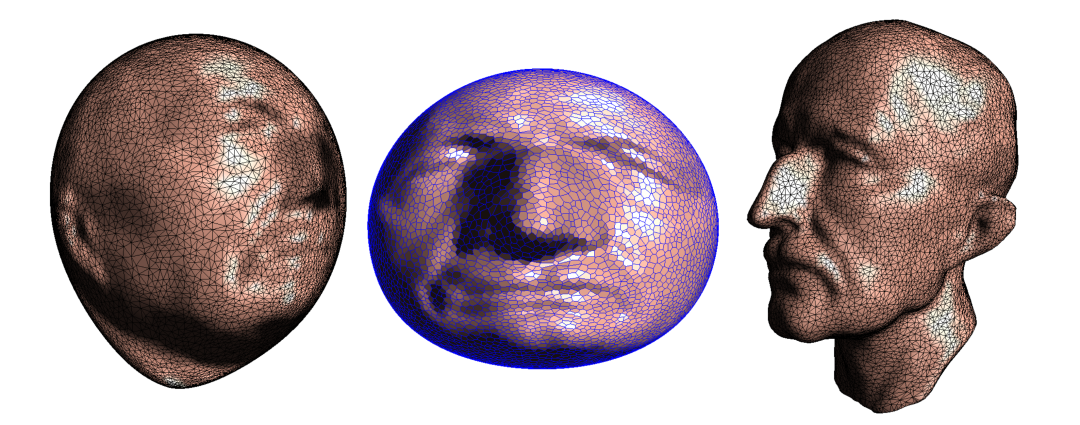
Below we use relatively rigorous mathematical language to accurately distinguish between "imagination" and "illusion". First, generative models are based on the data science principle of “manifold distribution”. The so-called "manifold" can be regarded as a high-dimensional generalization of surfaces. As shown in Figure 3, the Maitreya Buddha surface is a two-dimensional manifold embedded in a three-dimensional space. Each point on the surface requires three coordinates to describe, so the point is three-dimensional; suppose there is an ant crawling on the surface. At each point, the ant's activity direction has only two degrees of freedom, so the surface is two-dimensional. As shown in the figure, we can continuously map the surface to a two-dimensional plane, and any point on the surface corresponds to a point on the plane, thereby achieving dimensionality reduction. Furthermore, there is a probability distribution on the surface, which is represented by sampling points on the surface. It is mapped and pushed to the plane, and becomes a probability distribution on the plane area, which is represented by sampling points on the plane. In turn, surfaces and measures in the original three-dimensional space can be represented by mapped and planar data.
|
|
|
Figure 3. Maitreya curved surface and its embedding on a flat surface.
As shown in Figure 4, we examine LeCunn's MNIST handwritten digit training set. Each sample is a 28x28 gray value image that LeCunn scanned from an envelope. It can be abstracted into a point in a 784-dimensional space. The MNIST data set contains a limited number of discrete points, forming a discrete point set (also known as a point cloud). Any point in the image space is a grayscale image, but only a small part of it is a handwritten digital image, that is, this subset is. A discrete point set is a discrete sampling of . If the sampling density is sufficient, the topological and geometric properties of . Hinton's work verified that it is a two-dimensional manifold (that is, a surface) embedded in a 784-dimensional image space. In the right frame of Figure 4, Hinton's t-SNE algorithm will map to the plane. This mapping is a continuous bijection (topological homeomorphism), from the data manifold to the latent space, which is called encoding mapping (encoding). The image of each image sample is called a latent variable, or feature vector. It is called a decoding map that transforms each latent variable into the original image.
|
|
|
Figure 4. LeCunn’s MNIST training set; Hinton’s t-SNE dimensionality reduction.
Furthermore, we examine 10 handwritten numbers from 0 to 9. Each number corresponds to a probability distribution on the data manifold. Its density function is, and the support set of the probability measure is recorded as,
Obviously, each image represents a unique number, so the supports do not overlap with each other. The encoding mapping will be mapped to the latent space, and the probability measure will be pushed forward to the latent space to become, which is called the latent data distribution. is the support set of the latent data distribution: let it be any measurable set, then its measure is defined as
It can be seen from the figure that the implicit distribution branches are separated from each other and are separated by large gaps. Then the original data manifold and the original data distribution can be represented by the encoding and decoding mapping and the latent space data probability distribution,
So, how to represent the encoding and decoding mapping sum in the AI generation model? The answer is the "law of universal approximation" of deep neural networks. Kolmogorov and Arnold proposed the Kolmogorov-Arnold representation theorem in the process of proving Hilbert's 13th problem: any continuous multi-variable function can be represented by a finite composite of a single-variable continuous function and a binary addition operator. Deep neural network is essentially the computer implementation of this theorem. Whether it is CNN, DNN or Transformer, it remains the same. Theoretically, if there is a continuous mapping, then for example there is a Kolmogorov-Arnold approximation, that is, for any, there is a deep neural network approximation with an error less than .
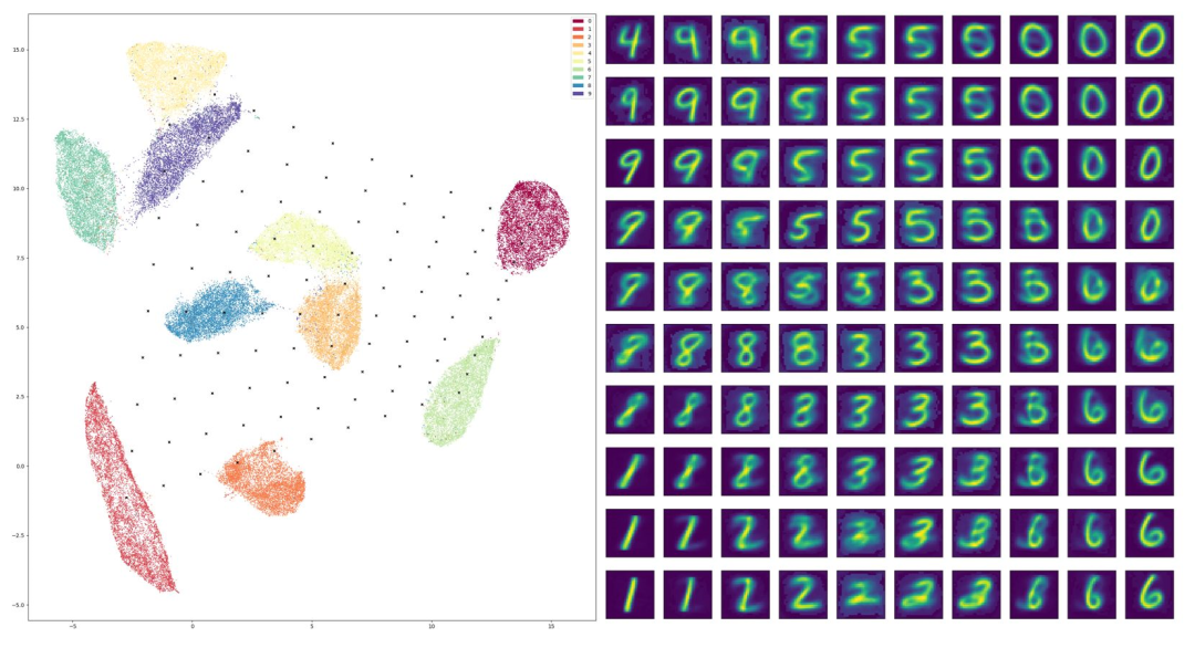
Figure 5. UMap embedding and sampling.
So does it exist theoretically? Whitney's manifold embedding theorem asserts its existence: any smooth, dimensional real manifold can be smoothly embedded into a dimensional Euclidean space. The author believes that the currently widely circulated manifold dimensionality reduction algorithm UMap is essentially inspired by the proof of Whitney's manifold embedding theorem. First, we find a family of finite open covers for the manifold, here an open set, which can be locally embedded in (for example, using the principal component analysis PCA method). We construct a partition of unity for finite coverage, and then use unit decomposition to paste the local embedding into a global embedding, embedding the manifold into a very high-dimensional Euclidean space. Then Whitney applies techniques to project the embedded image of the manifold into a co-one-dimensional subspace randomly. Whitney said that the projected image is still embedded with probability one (that is, there is no self-intersection), so that we embed the manifold into it. By repeatedly using Whitney's technique and constantly projecting, Whitney said we can guarantee reduction to dimensionality.
Figure 5 shows that we use UMap to reduce the dimensionality of the MNIST surface to a planar latent space. There are a total of 10 supports of the latent data distribution. We sampled 100 feature vectors in the latent space and generated the corresponding images through decoding mapping. We see that if the latent feature vector falls in the supports of the latent distribution, the generated image can clearly identify the numbers; if the latent feature vector falls in the blank space between the supports, the generated image is blurred and difficult to identify. This condition is called pattern confusion and is a common hallucination. It can be seen that if the data distribution is learned inaccurately, erroneous output will be produced and hallucinations will occur.
Generate model framework
So, how to represent the latent space data distribution in AI generative models? (here,). The answer is the reversible transfer transform, here is a known probability distribution, such as the uniform distribution inside the unit ball, the Gaussian distribution of the entire latent space, any probability distribution that can be generated by a computer pseudo-random number algorithm, usually called white noise. The transfer transformation will map to,transform the probability distribution into,i.e. Since it is known, a representation of the distribution of the data is given. As shown in the figure, the left frame is a uniform distribution within a rectangle, with a cell decomposition, and each cell is marked with a different color; the right frame is the hidden data distribution of MINIST, with corresponding supports. The transfer mapping maps the cells on the left to the supports of the same color on the right, and maps the boundaries of the cells to the boundaries of the supports (the gaps between the supports are ignored by the transfer map). Once again, the Kolmogorov-Arnold representation theorem can be approximated by deep neural networks, whereby the AI model can fully express arbitrary data distributions.
From this, we see that according to the manifold distribution rule, the training set essentially samples the data manifold to approximate the data distribution. The AI generation model has learned two things: 1. Use encoding and decoding mapping to express the data manifold; 2. Use transmission mapping to express the data distribution. According to the Kolmogrov-Anorld representation theorem, both encoding and decoding mapping and transmission mapping are approximated by deep neural networks. Combining these modules, we obtain a framework for general generative models.
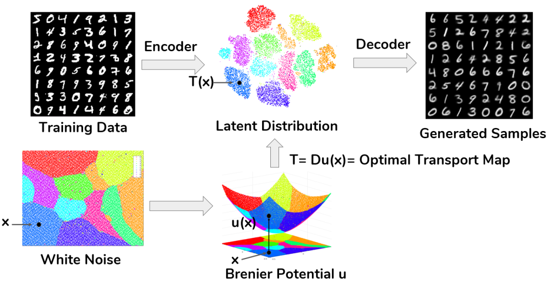
Figure 6. Framework of the generative model.
As shown in Figure 6, the training process of the generative model is as follows: we first use the training set to train to obtain the encoding and decoding mapping, and then obtain the transmission mapping through training. The reasoning process of the generative model is as follows: white noise conforming to the distribution is generated by the computer, assuming that one of the samples is; the transmission mapping maps the sample into the hidden support set; the decoding mapping maps the latent feature vector into a handwritten digital image.
The samples generated by the generative model are "imagination" if the sample falls on the data manifold and fall within the support (or edge) of the data distribution; the samples generated by the generative model are "illusion" if the sample falls outside the support of the data distribution.
Causes of “hallucinations”
However, the current mainstream in the AI field has ignored the premise of the Kolmogorov-Arnold representation theorem: the approximated mapping must be continuous, that is, the usual deep neural network can only express continuous mapping. The work of 2018 Fields Medal winner Alessio Figalli shows that under normal circumstances, transmission mapping is not a continuous mapping, there are singular sets in it, and the mapping is discontinuous. Therefore, deep neural networks cannot accurately express transfer maps. The inability to accurately learn and represent data distribution is the core cause of hallucinations.
First, Brenier's polar decomposition theorem asserts that all transfer maps that satisfy can be decomposed into a composite of two maps: , here is the optimal transfer map from to , satisfies natural boundary conditions, and is a measure-preserving map. The same Arnold regarded all volume-preserving (Pauleberg measure) diffeomorphisms as an infinite-dimensional Lie group, and the Euler equation of an ideal incompressible fluid became a geodesic equation on this infinite-dimensional manifold, thereby providing a geometric and topological framework for theoretical fluid dynamics.
The optimal transmission mapping here is defined as follows: all transmission mappings are examined and satisfied, and the total transmission cost is defined as:
The one with the smallest total transmission cost is called the optimal transmission mapping. Brenier's theorem asserts the existence and uniqueness of the optimal transmission map, and the optimal transmission map is equal to the gradient of a certain convex function (Brenier potential energy function), and the Brenier potential energy function satisfies the Monge-Ampere equation (Monge-Ampere Equation)
Here, is the density function. The Monge-Ampere equation is a strongly nonlinear elliptic equation.
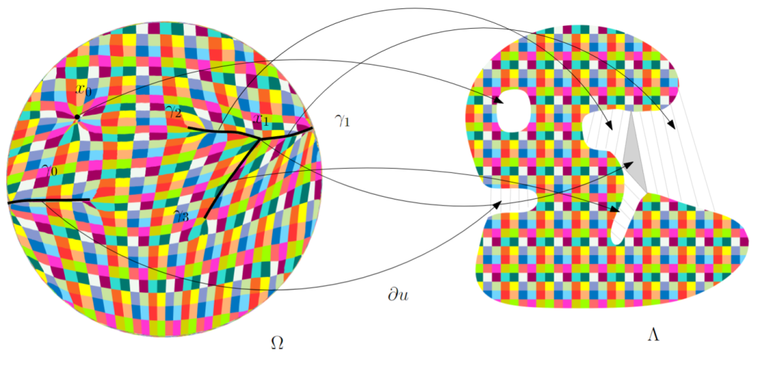
Figure 7. Counterexample given by Figalli, the transmission map is discontinuous.
Figalli gives an example, as shown in Figure 7. We examine the optimal transmission mapping from the uniform distribution inside the flat disk to the uniform distribution inside the irregular area on the right. The black curve inside the disk represents the singular set, and the optimal transmission mapping is discontinuous on the singular set. From the perspective of the Brenier potential energy function, it is smooth almost everywhere, but it is only continuous and not smooth on the singular set, so it is discontinuous on the singular set. This optimal transmission mapping cannot be expressed directly using deep neural networks.
If we can calculate the Brenier potential energy function, we can calculate the optimal transmission map and find the singular set, which corresponds to the boundary of the support. If there are multiple connected branches, , that are separated from each other, then the singular set under the generalized gradient map will look like the gap between the covers. Therefore, if we can accurately solve the optimal transmission map, we can accurately find the boundaries of the support of the data probability distribution. And calculating the optimal transmission map boils down to solving the Monge-Ampere equation.
Figure 8. Minkowski problem: The convex surface is governed by Gaussian curvature and can be reduced to spherical optimal transmission.
As early as 1993, Mr. Qiu Chengtong proposed hundreds of open problems in the field of differential geometry, one of which was the invention of numerical methods to solve the Minkowski problem. This problem is a rigidity problem in convex geometry: how to restore the shape of a convex surface through Gaussian curvature. This problem can be transformed into a spherical optimal transmission problem, which ultimately boils down to solving the spherical Monge-Ampere equation. Mr. Qiu guided the author's team to solve the optimal transmission problem in Euclidean space through the geometric variation method in 2013. In 2019, he developed an algorithm for solving the optimal transmission problem on the sphere, thus solving this open problem. Using this method, we can accurately find the singular set and thus the boundary of the support of the data probability distribution.
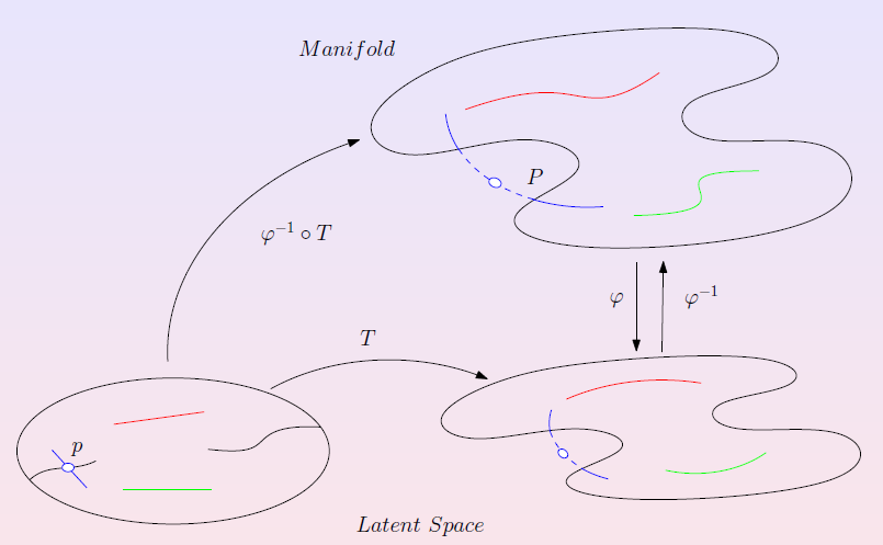
Figure 9. Data manifold edge detection experimental design.
We use this method to detect the edges of the data manifold. As shown in Figure 9, we designed a generation model for face color images. The image space dimension is three million and the latent space is about 150 dimensions. We use autoencoder training to obtain the encoding and decoding mapping sum, and then use the geometric variation method to obtain the optimal transmission map from the uniform distribution to the hidden data distribution, and obtain the singular set through the normal vector. We design several line segments in . Each line segment is mapped by transmission mapping into a curve segment in the latent space (red, green line segments), and then decoded and mapped into a curve segment on the data manifold. Each curve segment is a short video that transforms from one face into another. If the line segment (middle blue line segment) intersects the singular set (middle black curve), the curve on the data manifold will cross the boundary of the data manifold, and we will produce some face images that comply with physiological laws, but the probability of encountering them in real life is zero. Figure 10 shows such a curve. We start from the boy with brown hair and brown eyes and end with the blonde woman. In the middle, there is a face with one blue eye and one brown eye (a face with different pupils). There are no faces with different pupils in the training set. These faces with different pupils are at the edge of the face image manifold. They seem reasonable, but the probability of encountering them in real life is zero. This experiment shows the following points: a. There are edges in the data manifold, and samples not covered in the training set can be generated at the edges; b. The edges of the data manifold correspond to the singular set of optimal transmission mappings, which can be calculated using our geometric variation method; c. The edges of the data manifold are the most imaginative, and may also represent limitations of physical and biological laws, and should be treated with caution.
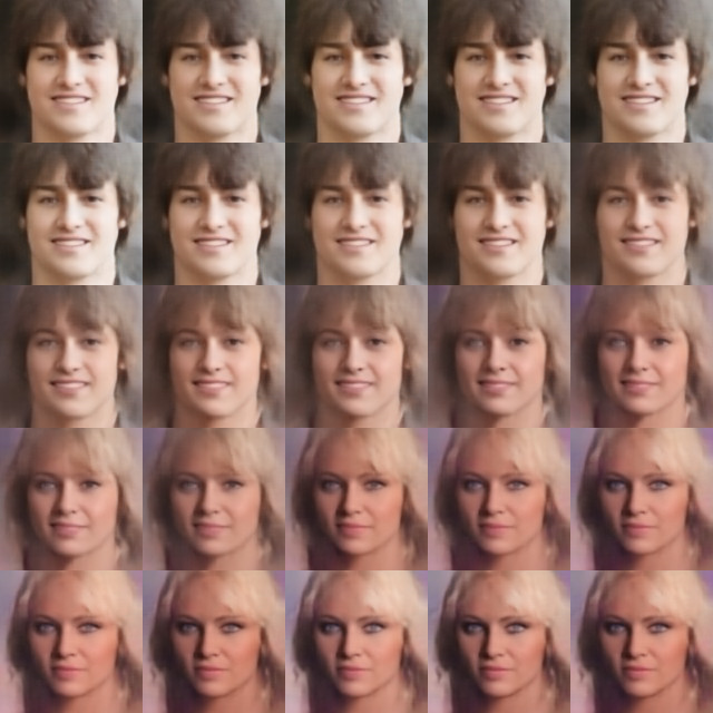
Figure 10. Face near the boundary of the face image manifold.
If we can accurately find the edges of the data manifold, and these boundaries represent the boundaries of natural laws, then we need to be careful not to cross the boundaries when generating samples to avoid the occurrence of hallucinations. For example, in the puppy video generated by Sora, all 3 puppy images form a probability distribution, and all 4 puppy images form another probability distribution. Due to self-occlusion, 4 puppies sometimes look like 3 puppies. These pictures are located at the boundaries and contacts of the support set, but the boundaries that the Sora algorithm cannot capture can easily cross, causing an illusion. The boundary here has a physical meaning and logically should not be crossed.
In the red wine video generated by Sora, the wine glass has two stable states: an upright state and a horizontally lying state, as well as a transition state from upright to pouring. It is easy for us to collect samples from steady states, so Sora generates steady-state images; it is very difficult to collect samples from transition states, so Sora does not generate transition state images. But for human perception, transition states are key to understanding physical processes. The boundary of the probability distribution support corresponding to the steady state is the transition state, and the sample generation of the transition state is crucial.
|
|
|
Figure 11. The non-smooth points of the Brenier potential energy function correspond to the singular set of the optimal transmission map and correspond to the boundary of the data distribution support.
Currently the most popular generative models are those based on diffusion processes. For any data distribution, the so-called entropy flow corresponds to the diffusion process. During the diffusion process, the entropy of the probability distribution increases monotonically and finally reaches the maximum value. Among the probability distributions given the expectation and variance, the one with the largest entropy is the Gaussian distribution. Therefore, the diffusion process is to give a transfer map from the data distribution to the Gaussian distribution. The diffusion process can be simulated by Langevin dynamics, that is, each particle adds a white noise random walk to achieve a Gaussian distribution. The advantage of the diffusion model is that there is no need to express the probability density explicitly, and all particles can walk independently in parallel in random fashion. However, its shortcoming is that it blurs the boundaries of the probability distribution support. The final transmission transformation (inverse diffusion) gives a low accuracy of the data distribution, cannot obtain the exact support boundary information, and generates samples outside the real data distribution, forming an illusion. This once again proves that the boundary of the data distribution support has biological significance and cannot be crossed at will in the task of real image generation.
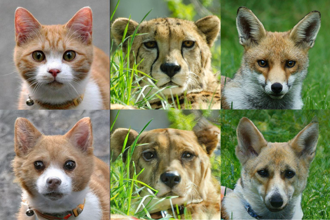
Figure 12. By grasping the boundaries of data distribution clusters, we can accurately synthesize cross-species organisms. Top row: real images of creatures; bottom row, from left to right: creatures between dogs and cats, dogs and leopards, dogs and foxes. (Written by Wang Zhanpeng)
As shown in Figure 11, we use the geometric variation method to calculate the optimal transmission mapping and obtain the Brenier potential energy function. Through the non-smooth points of the potential energy function (points where the normal vector mutates), we can obtain the singular set of the transmission map (black curve in the right frame). The singular set corresponds to the boundary of the data probability distribution support. As shown in Figure 12, by grasping the boundaries of the data distribution support, we can accurately synthesize cross-species organisms. The upper row of the picture is a real biological image. We find the data distribution edges of images of different species, then find the shortest connection between the distribution edge of cats and the distribution edge of dogs, and generate an image between cats and dogs along the connection line, as shown in the lower left corner. Likewise, we can generate creatures that are somewhere between a dog and a leopard, or a dog and a fox. This shows the imagination and generalization ability of this method.
In the currently popular Vincentian graph application, the image generation model and the large language model are combined to establish a mapping between the image latent space and the semantic latent space, which can map from the language prompt to the image latent space, thereby generating images according to the prompt. People introduce the token concept of language model into the image field, decompose the image into many sub-images as tokens, and then use the tokens as samples for training. As shown in Figure 2, although each generated token looks very realistic, the probability distribution between tokens is not accurately learned, so although the generation quality is high locally, it is seriously distorted overall. This requires us to strengthen the learning of joint probability distributions between tokens, that is, the learning of token context probability distributions. We can regard all possibilities of each token as a token data manifold. The images composed of all tokens constitute the image data manifold. The image data manifold is the product manifold of the token data manifold. The joint probability distribution between tokens is defined on the product manifold, thereby constructing a hierarchical learning structure to reduce illusions.
Summary
Generative large models can be explained from the perspective of differential geometry using the manifold distribution principle: each data sample is regarded as a point in the high-dimensional background space; the set of all data samples can be described as a point cloud in the background space, contained in a certain low-dimensional data manifold, the manifold dimension is much lower than the background space dimension; at the same time, the data sample set has a specific probability distribution on the data manifold. The training process of large models can be summarized in the form of differential geometry as: 1) learning the topological geometric structure of the data manifold; 2) learning the probability distribution of the data on the manifold. The inference process of large models is summarized as sampling on the data distribution. The topological geometric structure of data manifolds is usually represented by encoding and decoding mappings; Whitney manifold embedding theory guarantees the existence of mappings, and the UMap algorithm imitates the proof of the theorem; data probability distribution is usually represented by transmission mapping: transmission mapping maps the known Gaussian white noise to the data distribution.
Deep neural networks can universally approximate any multivariate continuous function. The current various deep neural networks CNN, DNN, and Transformer are all algorithm implementations of the Kolmogorov-Arnold theorem. The K-A theorem proves that any multi-variable, continuous function can be represented by a finite-order composite of a single-variable function and an addition operator; however, the K-A method cannot directly represent discontinuous functions; the encoding, decoding mapping and transmission mapping in the current AI generation model are represented by deep neural networks. However, the work of Fields Medal winners Villani and Figalli pointed out that the transmission map is discontinuous and the current AI generation model cannot accurately learn it. Probability distribution support set boundaries represent the limits of natural laws, which often have physical, biological or mathematical significance and are insurmountable in nature. The traversal behavior of traditional generative models creates illusions. The diffusion model turns the data distribution into a Gaussian distribution, which is a rough approximation, blurring the boundary information of the data distribution support set, and causing pattern confusion and hallucinations.
The AE-OT (AutoEncoder-OptimalTransport) generation model proposed by Mr. Qiu and the author's team is expected to fundamentally overcome the problems of mode collapse, mode confusion and hallucination. The AE-OT generation model decouples the topological structure learning task of the data manifold and the learning task of the data probability distribution. The former uses AI methods such as Auto-Encoder, and the latter is implemented using the geometric variation method we invented to solve the optimal transmission problem. AE-OT can accurately obtain discontinuous probability distribution transmission transformation (rather than rough approximation), and strictly determine the boundary of the probability distribution support set. The AE-OT model itself avoids crossing the boundary of the probability distribution support set during the generation process, theoretically ensuring that fallacies are eliminated and illusions are prevented. The AE-OT model can be combined with existing generation models to provide accurate data probability distribution information, warn when the generation process is close to the edge of the distribution, and prevent hallucinations.
Optimal transmission theory seeks the most economical method to achieve transformation between probability distributions. Brenier's polar decomposition theorem asserts that any transmission transformation can be decomposed into the optimal transmission transformation and the Pauleberg volume transformation, so the optimal transmission transformation determines the continuity of the entire transformation. Brenier's theorem boils down the optimal transmission problem to solving the strongly nonlinear Monge-Ampere equation. Mr. Qiu Chengtong proposed more than 100 open problems in differential geometry in 1993, including solving the Minkowski problem, which is equivalent to solving the spherical Monge-Ampere equation. In 2013, the team of Mr. Qiu and Professor Gu proposed a solution algorithm for the Monge-Ampere equation using the principle of geometric variation; in 2019, they solved the Minkowski problem-the optimal transmission problem. This theoretical result is directly used to improve the quality of AI generative models.
Historical development will allow us to see that geometric analysis is providing a rigorous and solid mathematical foundation for generative AI. With the guidance of causal logic, probabilistic models are expected to eliminate AI illusions from the source.
Machine-translated from the Chinese original 用微分几何理论破解AI幻觉 (published 2025-09-02). WeChat original ↗